EMPIRICAL ECONOMIC BULLETIN


THE CENTER FOR CLOBAL AND RECIONAL ECONOMIC STUDIES BRYANT UNIVERSITY

EEB--UNDERGRADUATE ECONOMICS JOURNAL f--..... f �'-'"•fl.'IC,NI \ t �--· ___,
Hit I •
--- '
 EDITOR: Ramesh Mohan
DESIGN & LAYOUT: Ramesh Mohan and Rebecca Marcus
MISSION STATEMENT: The Empirical Economics Bulletin is the undergraduate journal for the Department of Economics, Bryant University. The journal is produced in conjunction with the Bryant Economic Undergraduate Symposium. The focal point of the Symposium is on training undergraduate students in the art of writing, presenting, and publishing empirical research papers on a range of socio-economic and economic topics. The Symposium’s primary emphasis is empirical studies with policy relevance. Students are then able to publish their empirical papers in the Empirical Economics Bulletin. An objective of the Economics’ Department, Bryant University is to train students to conduct quantitative economic data analysis and to present the results in a coherent and meaningful way. This objective is met through having the Symposium and the publication of the Empirical Economics Bulletin. The first issue was in Spring 2008 and has been published annually with original work from an array of student authors.
SUBMISSION GUIDELINES: Students may submit their socio-economic and economic work here: Ramesh Mohan at rmohan@bryant.edu. Limit one submission per author. Each submission should have a title page with the title; name of author; abstract; keywords; JEL classification; author’s email. Previously published work is not accepted. The reading period is September 1 to December 1. Copyright reverts to author upon publication.
Any questions may be directed to Professor Ramesh Mohan at rmohan@bryant.edu.
© 2022 Empirical Economics Bulletin
Table of Contents Effectiveness of Aid: Panel Data Analysis of Foreign Aid in Africa, Will Bittrich 1 Impact of Corrup�on on Economic Growth in Central America: A Panel Data Analysis, Ben Bresnee …… 13 Determinants of Real Median Household Income in the United States Using Time-Series and Panel Data Analysis, Evan Clark ..................................................................................................................................... 25 A Panel Data Analysis on Income Inequality on Life Expectancy in Asia, Julianna Flaccavento 43 The School-to-Prison Pipeline: A Panel Data Analysis, Samuel J. Guider …. 63 The Empirical Analysis of Motherhood Penalty: The Effect of Having Children on Women’s Career, Madison Henry 85 A Panel Data Analysis of Ins�tu�onal Quality, FDI, and Public Debts’ Impact on Economic Growth for ASEAN, Joshua Kearney ..…………………………………………………………………………………………………………………… 104 An Empirical Analysis on Dispari�es in Access to Healthcare in New York City, Olivia Lemire .. 119 Panel Data Analysis: Gender Wage Gap and Macroeconomic Factors Impacts, Yuzhe Lin …………………. 134 The Effect of Minimum Wage Increases on Employment of Teenagers in New England, Felicia O’Reilly 142 Panel Data Analysis of Import Tariff Policy on Economic Growth and Industrial Output in Developing Economies, Connor A. Palazzo .. 159 A Panel Data Analysis of the Effects of Macroeconomic Variables on Income Inequality in La�n American Countries, Scot Poretsky …………………………………………………………………………………………………………………. 171 Causal Rela�onship Between Defense Spending and Economic Growth in Countries with Different Income Levels, Kyle Sampson 188 Interna�onal Integra�on and Export-Led Growth in La�n America: A Panel Data Analysis, James Titus . 203 Granger Causality of the Rela�onship Between Tourist Flows and Household Expenditure in Jamaica, Ben Williams ……………………………………………………………………………………………………………………………………………. 215
Effectiveness of Aid: Panel Data Analysis of Foreign Aid in Africa
Will Bittrich
Abstract:
This paper investigates the effectiveness of international foreign aid flows into the continent of Africa. The study incorporates economic information into an econometric model to examine the influence of variables including natural resources, types of government, corruption, and education. The influence of gender equality and rule of law in relation to developed countries is factored in through a dependent variable. These findings provide an analysis on the efficiency of foreign aid and its effects on economic development in the region.
JEL Classification: H7, I3, F35
Keywords: Foreign Aid, Intergovernmental Relations, Poverty
Economics Student, Bryant University, 1150 Douglas Pike, Smithfield, RI 02917. Phone: (781-715-4091). Email: wbittrich@bryant.edu
1
Foreign Aid has become an increasingly contentious topic as a multitude of countries in Africa continue to diverge from the developed economies of the West. Cash payments, structuralized loans, and other subsidies have played a key role in development plans for decades, all which have had varying degrees of success. Attempts to effectively develop these nations in Africa have been constantly altered to suit our globalized world. Each nation in need has individual needs dependent on their resources, economy, and infrastructure, making the task of economic development a multidimensional issue.
This study aims to enhance understanding of how efficiently and effectively foreign aid is being used to help develop economies and enhance the quality of life of people living in these countries. From a policy perspective, this analysis is important because it can help identify the effective policies set by institutions such as the United Nations, developing nations, or other sovereign states responsible for many of the development projects internationally. The relevance of this study is to help contribute to the ongoing research regarding how to help the roughly 800 million people living in extreme poverty in Africa
This paper was guided by three research objectives that differ from other studies: First it investigates the possibility of institutional capacity as a nation using dynamic data; Second, it incorporates a multitude of national and international factors that could affect Foreign Aid; Last, it analyzes the relationship of Foreign Aid to institutional strength in relation to labor markets, economic freedom, and international aid.
1.0 INTRODUCTION
2
2.0 Foreign Aid to Africa
Figure 1 shows the breakdown of foreign aid payments internationally by continent. Using econometric techniques, the researchers identified recent trends of decreased aid flows towards the regions of Africa and Asia in the years leading up to 2016. The divestment is suspected to be due to the slight increase in aid towards Eastern European and South American countries also in need of capital. Moreover, aid has shifted greatly from debt relief to more social and economic purposes. Figure 2 identifies the trends of sectoral aid programs, drawing data from NGO’s, international agencies, and national aid programs.
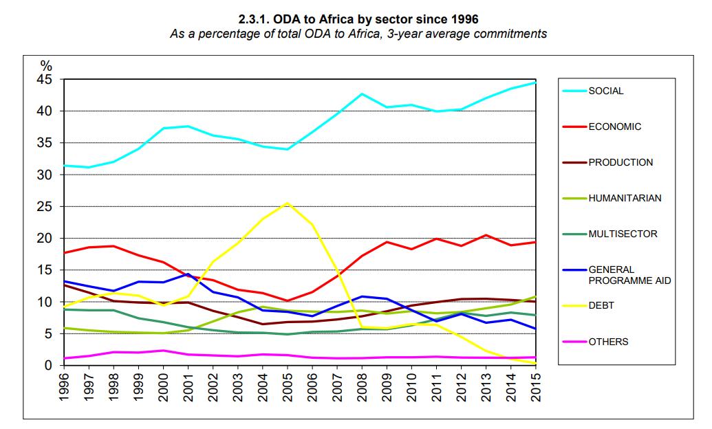
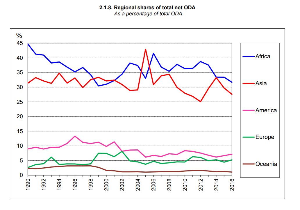 Figure 1: Yearly Foreign Aid Flows Internationally
Figure 2: Yearly Foreign Aid by Sector
Figure 1: Yearly Foreign Aid Flows Internationally
Figure 2: Yearly Foreign Aid by Sector
3
Source: OECD, (2018)
3.0 LITERATURE REVIEW
Foreign aid has become a contentious issue in the past decades due to repeated failures and continuing divergence of many developing nations, specifically in subSaharan Africa (Kamguia, Tadadjeu, Miamo, et al 2022). Despite foreign aid almost tripling from 1970’s to the 1990’s, growth in Africa remained relatively stagnant. (Easterly, 2005) identifies this issue as not a lack of capital, rather an absence of responsibility from the wealthier nations to ensure effectiveness of development. He states that the quality of aid is being overlooked for more quantity-oriented marketing campaigns, where it delivers the “feel good” moment the public desires. While there are a multitude of reputable arguments criticizing the application and effectiveness of aid, (Moyo, 2011) suggests that aid has had a net negative effect on the continent Citing that Africa has diverged further, increased its debt load, increased civil conflict, and caused more volatile inflationary periods because of aid.
The debate over the application and effectiveness is what dominates the discourse regarding aid internationally and within development agencies. (Brautigam and Knack, 2004) argue that the central issue is of bad governance, citing that no matter the amount of aid if it is not allocated to trustworthy or qualified hands it will continue to be ineffective. The issue of governance can be attributed to a multitude of factors such as colonialism, indigenous institutions, and civil conflict. Contrary theories to identify the specific factors inhibiting aid have risen, (Andrews, 2009) claims that the focus on macro-economic factors have hindered development and believes that smaller sociocultural factors may be the root cause. Overall, the effectiveness of aid is a developing
4
argument with studies being constructed and cited to identify new trends in the effort to alleviate millions from poverty.
4.0 DATA AND EMPIRICAL METHODOLOGY
The study uses annual panel data from 2000 to 2020. Data was obtained from the World Development Banks (IRDB) website on World Development Indicators. Publicly available World Bank data excludes countries that are viewed as developed and in this study, I will only be using 20 countries in the African region. Shown below is the econometric model, ordinary least square regression, fixed effect regression, random effect regression, and the Hausman test results.
Model:
4.2 Empirical Model
I followed the Hongli and Vitenu-Sackey (2020) model for the relationship between foreign aid and development indicators.
The model:
There are six independent variables in the model, each with an individual relationship to the dependent variable of lnGDP Per Capita. Appendix A and B provide data source, acronyms, descriptions, expected signs, and justifications for using the
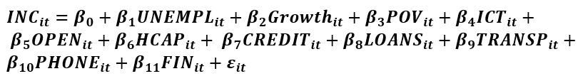
LnGDP Per Capita = β0 + β1 Rent + β2 SECEDU + β3 FDI + β4 WOMIDX + β5 BRDMONY + β6 BIRTHS + β7 HIV + β8 FAID + ε
5
variables. LnAid is the annual flow of foreign aid from international institutions and individual countries to the nation. It represents the total allocation of capital being transferred for development purposes. HDI represents the United Nations Development Project’s Human Development Index which is a measurement of average achievement in key dimensions of human development. Rule of Law is derived from the World Justice Project’s index that measures the perceived effectiveness and application of laws in the country. Corruption is reflected by the authors estimate of corruption control, indicating how many citizens believe that there is corruption in their government. Voice equality is a control variable used to identify freedom levels of press and speech. Lastly, Government Effectiveness is a proxy for the country’s ability to collect taxes, provide public goods, and implement policy.
The dependent variable in this model is the natural log of GDP Per Capita, a proxy for economic growth. GDP Per Capita as calculated by the World Bank is the country’s yearly GDP divided by the country’s population. This figure is associated with economic growth, although it does not necessarily reflect the distribution of the growth. The proxy is broad but provides a reliable macro-economic indicator for the nation’s economic success year over year. Studies such as Easterly (2005) and Acemoglu and Robinson (2010) utilize GDP Per Capita in models to identify growth patterns.
5.0 EMPIRICAL RESULTS
The results estimated by the model are presented below in Table 2, with Ordinary Least Squares, Fixed Effect, and Random Effect outputs presented. After performing the
6
Hausman test, I identified the Fixed Effect model to be the most accurate estimator for this data set.
Note: ***, **, and * denotes significance at the 1%, 5%, and 10% respectively. Standard errors in parentheses
The most statistically significant variables are the Women’s Index, Birth Rate, Foreign Aid, and Secondary Education. Specifically, the WOMIDX variable was statistically significant at the 1% level, Hongli and Vitenu-Sackey (2020) also found high levels of significance in the Women’s Index variable proxy through their estimations.
Birth Rate and Secondary Education are also both statistically significant at the 1% level, with education representing the largest variable difference of 484.60. Foreign Aid holds a
FDI Model OLS Fixed Effect Random Effect RENT -22.06* (9.64) -1.70 (3.77) -4.29 (2.77) SECEDU 611.05*** (109.83) 484.60*** (178.32) 720.29*** (199 13) FDI 1.06* (3.58) .896* (.231) 9.37** (2.34) WOMIDX 18.92*** (4.73) 26.29*** (5.33) 25.06*** (5.08) BRDMNY 3.73 (2.55) 12.48* (4.96) 11.59* (4.49) BIRTHS -317.02*** (39.33) -77.43*** (10.82) -63.86** (12.37) HIV -.280* (.00927) -.116 (.0017) -.083* (.0015) FAID 14.77** (6.90) 22.15** (7.87) 19.32* (6.33) R2 6378 6211 5952 Number of obs. 394 394 394
Table 2: Regression results for African Aid Panel-Data
7
lower statistical significance at only a 5% level but still holds a relevant impact on the independent variable. Estimators that negatively affected GDP Per Capita were Birth Rate, HIV, and Resource Rents, with Birth Rate having the largest coefficient of -77.43. The variables that were not statistically significant to the 5% level were Resource Rents, Foreign Direct Investment, and HIV cases.
Examining these results, we find several trends and impacts of variables within the model that give us insight to the estimator’s significance. Increases in the variable Secondary Education had a large impact on GDP Per Capita, showing the correlation between increases in education and economic development. Alternatively, the second largest coefficient was the Birth Rate variable. Increases in birth per woman have negatively affected the GDP Per Capita of the entire population possibly due to the responsibility of raising children instead of participating in the workforce. Other notable estimators are the Women’s Index, where increases in the equality of genders results in a positive impact on GDP Per Capita. Additionally, Foreign Aid’s significance and coefficient is relatively low compared to other variables. This may be attributed to inefficient applications of aid, lackluster programs, or corruption within a country.
5.0 CONCLUSION
To conclude, this study attempted to expand on the literature presented identifying factors relevant to the development of African nations. I found there to be a statistically significant impact of increases in secondary education, foreign aid, and gender equality to increases in GDP Per Capita. Moreover, I found negative statistically significant impacts of increases in the Birth Rate on GDP Per Capita. Several coefficients that were not
8
significant to the 5% level were Resource Rents, Foreign Direct Investment, Broad Money, and HIV cases. Identifying indicators of economic growth in developing African countries is only one aspect of the research and it has several limitations. This study’s limitations include the use of proxy variables for variables with insufficient data points, exclusion of countries from the panel data set, and exclusion of possibly significant indicators from model. Nevertheless, the results of this study reinforced several empirical studies, Hongli and Vitenu-Sackey (2020) and Acemoglu and Robinson (2010). This research validated the impacts of variables such as the importance of education and institutional equality found in these studies Aid is a controversial and difficult concept to apply effectively to promote positive economic and social outcomes. The weaker relationship of GDP per capita growth to foreign aid in my model may be due to the ineffective application of aid but can also include other factors such as civil war, political conflict, global recessions, and resource dependence. Overall, my model identified key variables that played a role in GDP per capita growth in developing African countries.
Appendix A: Variable Description and Data Source
Acronym Description
FDI Net inflows of investment to acquire a lasting management interest.
WOMIDX A rating of laws, regulations, and reform trends that advance women's economic empowerment.
FAID Total yearly foreign aid inflows through bilateral and multi-lateral institutions.
Data source
World Development Indicators
World Development Indicators
World Development Indicators
9
RENT Sum of oil rents, natural gas rents, coal rents, mineral rents, and forest rents.
BRDMNY Measure of the amount of money, or money supply, in a national economy.
SECEDU Average years of secondary education.
HIV Total amount of HIV cases in the country yearly.
BIRTHS Birth rate, crude (per 1000 people)
World Development Indicators
World Development Indicators
World Development Indicators
World Development Indicators
World Development Indicators
Appendix B- Variables and Expected Signs
Acronym Variable Description
What it captures Expected sign
FDI Foreign Direct Investment Total yearly inflows of lasting FDI +
WOMIDX Women’s Business and Law Index Gender Equality Nationally +
FAID Foreign Aid Total inflows of bilateral and multi-lateral aid
RENT Total Yearly Resource Rents Amount of money received from natural resource sales
BRDMNY Broad Money Rate of movement of money within an economy
+
-
+/-
SECEDU Secondary Education Average education levels in a country +
HIV Total Positive HIV Cases Health crisis issues within a country -
10
BIRTHS Birth Rate Average amount of children per female 11
BIBLIOGRAPHY
Acemoglu, Daron, and James Robinson. “The Role of Institutions in Growth and Development.” Review of Economics and Institutions, vol. 1, no. 2, 2010, https://doi.org/10.5202/rei.v1i2.14.
Andrews, Nathan. “Foreign Aid and Development in Africa: What the Literature Says and What the Reality Is.” Journal of African Studies and Development, vol. 1, Nov. 2009.
Bräutigam, Deborah A., and Stephen Knack. “Foreign Aid, Institutions, and Governance in Sub‐Saharan Africa.” Economic Development and Cultural Change, vol. 52, no. 2, 2004, pp. 255–285., https://doi.org/10.1086/380592.
Easterly, William. “National Policies and Economic Growth: A Reappraisal.” Handbook of Economic Growth, 2005, pp. 1015–1059., https://doi.org/10.1016/s1574-0684(05)01015-4.
Hongli, Jiang, and Prince Asare Vitenu‐Sackey. “Assessment of the Effectiveness of Foreign Aid on the Development of Africa.” International Journal of Finance & Economics, 2020, https://doi.org/10.1002/ijfe.2406.
Kamguia, Brice, and Miamo, Clovis, and Tadadjeu, Sosson, and Njangang, Henri “Does Foreign Aid Impede Economic Complexity in Developing Countries?” International Economics, vol. 169, 2022, pp. 71–88., https://doi.org/10.1016/j.inteco.2021.10.004.
Moyo, Dambisa. Dead Aid: Why Aid Is Not Working and How There Is Another Way for Africa. Penguin, 2011.
12
Impact of Corruption on Economic Growth in Central America: A Panel Data Analysis
Ben Bresnee
Abstract
This paper investigates the possible impact of corruption on economic growth in Central America. This study incorporates information into a model to examine the influence of different factors such as population growth, aid, human capital, gross domestic investment, Corruption, and consumption. This study finds that there is a negative effect of corruption on economic growth in Central America.
JEL Classification: O40, O50
Keywords: Corruption, Economic Growth
a Department of Economics, Bryant University, 1150 Douglas Pike, Smithfield, RI02917. Phone: (617)-875-0457. Email: benbresnee@gmail.com.
13
1.0 INTRODUCTION
There has been a lot of debate over the years on if corruption has an impact on economic growth. Two theories have emerged to describe how corruption influences economic growth. The first is called “grease the wheels” hypothesis which explains that corruption has a positive impact on economic growth since it promotes efficiency since the private sector can get around regulations. The second is called “sand the wheels” hypothesis” which explains that corruption has a negative impact on economic growth because it suggests that there will be less investment in a country with high corruption.
This study aims to enhance understanding of how corruption affects economic growth in Central America through indicators such as GDP per capita, gross fixed capital formation, government expenditures, population growth, official aid received, GNI per capita, and the Corruption Perception Index. This study specifically investigates the countries of Central America and the affects of corruption on economic growth. From a policy perspective, this analysis is important because it provides information on whether a countries level of corruption is affecting its growth. This will not only help the people of that country formulate policies but also other countries and their decisions on wanting to give aid to areas with high level of corruption or use the money more efficiently.
The rest of the paper is organized as follows: Section 2 gives a brief analysis of the trends in Central America surrounding corruption and economic growth. Section 3 gives a brief literature review. Section 4 outlines the empirical model. Data and estimation methodology are discussed in section 5. Finally, section 6 presents and discusses the empirical results. This is followed by a conclusion in section 7.
14
2.0 TRENDS
Figure 1 shows the corruption perception index of every country in 2018. This displays the level of corruption of each country and how they compare to other countries. Their scale shows countries with low corruption levels in blue and progresses into red with countries with a higher level of corruption. The map shows us that some of the highest areas of corruption are in parts of Asia, Sub Saharan Africa, and Central America where this study focuses on. A major trend in this figure is that countries with high levels of corruption tend to have neighboring countries with the same level of corruption or close to it. We can see this with places like Europe and Central America. In Europe, almost all of the countries have a CPI of 0-59 meaning there is low levels of corruption in these countries. On the other hand, if we look at Central America, we see the complete opposite. Each of their CPI is from 65-100 indicating that there are high levels of corruption in these neighboring countries.
Source: Transparency International
 Figure 1: Corruption Perception Index 2018
15
Figure 2 shows how people on Central America shows what percentage of the population thinks different groups and institutions are corrupt. As you can see the top three areas people think corruption is at its highest is in the police department, elected representatives, and the local government. Almost half the population believes that these groups are fully corrupted. This is because in Central America, organized crime and drug trades run rampant throughout the region. This is because police officers and elected officials tend get bribed to let these illegal actions take place.
Source: Transparency International
Figure 3 shows the correlation between CPI and development level using real GDP per capita Here it shows us that there is a negative corelation between CPI an the development level. Countries with high levels of corruption tend to have a lower development level while countries with low levels of corruption tend to have a high development level. This supports the “sand the wheels” hypothesis that corruption tends to slow growth in a country. This hypothesis suggests that because companies and civilians need to bribe people of power to be able to get what they want, there will be less investment which will slow down economic growth.
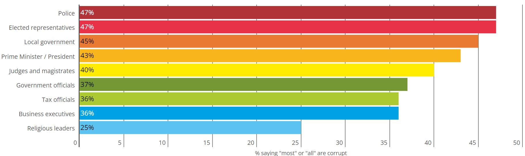 Figure 2: Corruption of Different Groups in Central America
16
Source: Grundler and Potrafke (2019)
3.0 LITERATURE REVIEW
Corruption affects countries all over the world. There has been a debate on whether it actually helps a countries economic growth or slows it down. Grundler and Potrafke
(2019) examined the effects of corruption on economic growth. They concluded that there is no evidence to suggest that corruption has any positive impact on economic growth but the complete opposite. They found that it has a negative effect on growth since it steers money away from investment into the country. A study done by D’Agostino et al. (2016) analyzed where countries with high corruption were spending their money on. Since they don’t use it as investment into the economy this study found that a lot of these countries put it into their military. Due to the fact that they spend a lot of their money on their military, this study concludes that corruption does have a negative impact since a big portion of it goes into the military which did not have an impact on economic growth. A study done by Del Monte and Papagni (2001) suggest similar results. They concluded that due to corruption, their will be a negative effect on growth
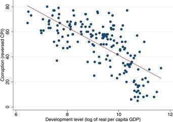 Figure 3: Correlation between CPI and Development Level
17
since governments have less money to spend on economic activities. There were two effects that they pointed out. The first being the effects corruption has on private investment and how it discourages it. The second effect is the efficiency of government spending. With corrupted leaders, government spending in these countries do not go into projects that will benefit the country but just for themselves. To dig a little deeper into the idea of corruption and the effects it has, Becker et al. (2009) did a study to show the effects of a country’s corruption on its neighboring countries. They found that countries with high levels of corruption influence other governments in surrounding countries negatively. They found that countries with similar political structures tend to influence each other and drive corruption up. This is similar to a previous graph where we saw that most of the high corrupted countries are surrounded by other highly corrupted countries. This shows that not only does corruption have an effect on a countries economic growth but it also has regional affects.
4.0 DATA AND EMPIRICAL METHODOLOGY
4.1 Data
The study uses panel from 2001 to 2020. The data was obtained from the Transparency International website and the World Development Indicators. In order to capture corruption in a country, this study uses the corruption perception index. Countries with a low score have high levels of corruption while a high score shows low levels of corruption. Central America is the focus of this study but because of the lack of data and no corruption perception index, Belize was excluded from this study.
18
4.2 Empirical Model
This research follows Chakravorty (2020) model to capture the effects of corruption on economic growth. Two variables were modified from the original model. First, to capture human capital, GNI per capita will be used. Second, gross capital formation will be used to capture investment. The model could be written as follow:
GDP= β0 + β1COR + β2INVES + β3C +β4POP + β5AID + β6GNI+ ε GDP is the annual growth of GDP in a country. It measures the growth rate by comparing the economic output of a country comparing it the the previous year. Independent variables consist of six var965iables obtained from various sources.
Appendix A and provides acronyms and descriptions First, COR represents the corruption level of a country. This data was obtained through the Transparency International website. The rest of the variables were obtained through the world Development Indicators. Second, INVES represents gross capital formation. Third, C represents general government final consumption expenditure as an annual percentage growth. Fourth, POP represents the population growth rate in a country. Fifth, AID represents the net official development assistance and aid given to a country. Lastly, GNI represents the gross national income per capita in a country.
5.0 EMPIRICAL RESULTS
After running the Hausman test, it showed this research should the fixed effect model. The empirical estimation results are presented in Table 1 It is important to note that the higher CPI score you have, the less corruption there is in that country. The empirical
19
estimation shows a positive relationship between corruption and economic growth at the 5% level. Although it is positive, what this really means is as a country increases its CPI score and becomes less corrupt, we expect economic growth to increase as well. The table also points out other factors that will affect economic growth. The results show that both gross capital formation and GNI per capita growth both are significant at the 1% level. Population growth is also significant at the 10% level. With these four variables being statistically significant, there are two that are not significant. Those being gross government consumption expenditure and development/assistance aid. Interpreting these results, it is evident that corruption does have a negative effect on economic growth. This does align with current literature to support the “sand the wheels” hypothesis. Not only does corruption have a negative affect but there is no evidence to show that development aid actually has an impact on economic growth. This could be due to the fact that since elected officials are seen as highly corrupt, when countries in Central America receive aid, they don’t use it for the benefit for the country but on themselves to better themselves off.
20
Table 1: Regression results for Central America
Note: *** , **, and * denotes significance at the 1%, 5%, and 10% respectively. Standard errors in parentheses
5.0 CONCLUSION
In summary, corruption in Central America has a big impact on the economy and people of those countries. The results suggest that corruption negatively contributes to the slow economic growth that Central American countries go through. It also suggests that things like gross capital formation and population growth have a positive impact while development aid has no impact at all. With these results come policy implications.
GDP OLS Fixed Random Corruption 1.853** (.847) 1.682** (.842) 1.853** (.847) Gross Capital Formation .0724*** (.009) .073*** (.009) .0724*** (.009) Gross Gov. Consumption Exp. -.0195 (.021) -.023 (.021) -.0195 (.021) Population Growth 1.074*** (.124) .768* (.410) 1.074*** (.124) Development assistance/aid -8.41e-13 (.000) 1.06e-09 (.000) -8.41e-13 (.000) GNI per capita growth .610*** (.039) .587*** (.040) .610*** (.039) Constant .483* (.261) .923 (.751) .483* (.261)
21
Corruption is hard to solve since the people solving it are the corrupted ones. This is why international organizations such as the UN should come and teach ethical practices in these countries. Only then will these elected officials be able to see that if they put money more towards things like investment instead of personal gain, their whole country can prosper and grow. This study adds onto the extensive research done by others that suggest the same results. Corruption has a negative impact on economic growth.
22
Appendix A: Variable Description
Variable Definition
GDP
Gross domestic product
COR
Measure of corruption in a country
GDPCAP GDP per capita
INVES Gross capital formation as a percentage of GDP
C Gross government consumption expenditure as a percentage of GDP
POP
AID
Population growth in a country
Net development assistance and aid received
GNI GNI per capita growth
23
BIBLIOGRAPHY
Gründler, K., & Potrafke, N. (2019). Corruption and economic growth: New empirical evidence. European Journal of Political Economy, 60, 101810.
d’Agostino, G., Dunne, J. P., & Pieroni, L. (2016). Government spending, corruption and economic growth. World Development, 84, 190-205.
Del Monte, A., & Papagni, E. (2001). Public expenditure, corruption, and economic growth: the case of Italy. European journal of political economy, 17(1), 1-16.
Alfada, A. (2019). The destructive effect of corruption on economic growth in Indonesia: A threshold model. Heliyon, 5(10), e02649.
Becker, S. O., Egger, P. H., & Seidel, T. (2009). Common political culture: Evidence on regional corruption contagion. European Journal of Political Economy, 25(3), 300-310.
Chakravorty, N. N. (2019). How Does Corruption Affect Economic Growth? An Econometric Analysis. Journal of Leadership, Accountability & Ethics, 16(4).
24
Determinants of Real Median Household Income in the United States Using Time-Series and Panel Data Analysis
Evan Clark
Abstract:
This paper’s main objective was to explore the determinants of income inequality using real median household income in the United States. This paper utilizes time series analysis to examine the Gini coefficient, trends in the top 1%’s share of wealth, and the relationship between real median income and varying demographics. The Gini coefficient is a summary measure of income inequality in a country. Income inequality is how unevenly income is distributed throughout a population. The results show that there is a negative correlation between the top 1%’s share of total wealth and the United States Gini rating, and that inequality in the United States has been steadily increasing. This study utilizes panel data analysis through fixed effects, random effects, and pooled ordinary least squares. The study observed the two determinants that had the most impact on real median household income were poverty, which was significantly negative, and human capital, which was significantly positive.
JEL Classification: D140, I320, J310
Keywords: Gini Coefficient, Income Inequality, Real Median Household Income
Economics Student, Bryant University, 1150 Douglas Pike, Smithfield, RI 02917. Phone: (267) 406-5052. Email: eclark4@bryant.edu
25
1.0 Introduction
Income inequality is a problem that not only effects transitional economies and developed economies, but the world at large in the past decades (Allison 2014). In accordance with the wealth hypothesis and Rubin & Segal (2015), as a country demonstrates economic growth they should also demonstrate a reduction in income inequality. This point however is a misconception, as most countries (the United States included) that have experienced economic growth, have not elicited the corresponding decrease in income inequality, thus leaving the question as to why ultimately unanswered.
This study seeks to resolves the unanswered questions regarding the relationship between economic growth and income inequality utilizing a methodology that mirrors Tsaurai (2020). In their work Tsaurai contradicts the preexisting theoretical literature conducted by Ayala et al (2001); Rubin & Segal (2015); Kaplan & Rauh (2010); Balassa (1978); Jacoby (2000); and Stiglitz (1998). Their rationale for doing so is that much of the existing work on income inequality only examines the issue from a single perspective lens and fails to acknowledge the exhaustive list of potential determinants. In addition to the issue noted by Tsaurai, it has also been observed that much of the current literature possesses a misconceived notion that there is a linear relation between determinants making it acceptable to generalize them, this is an issue that is addressed.
The area in which this paper differs from the literature of Tsaurai (2020), is that while they were focusing on the determinants of income in equality in transitional economies, this study analyzes the developed economy of the United States.
2.0 Income Inequality in the United States
Figure 1 shows the breakdown of the Gini Coefficient by country (World Bank 2022). The Gini Coefficient is defined based on the Lorenz Curve in which the percentiles of population according to income or wealth are graphed against the cumulative income or wealth of a population. The Gini Coefficient ranges from zero to one (often written as a percent) where zero is perfect equality, with every person earning the same amount, and one is perfect inequality, where a specific sect or group of people controls all of the wealth or income in a country and everyone else has nothing. Currently the top five countries with the lowest Gini Coefficient are
26
Slovenia (24.6), Czech Republic (25.0), Slovakia (25.0), Belarus (25.3), and Moldovia (25.7).
The United States on the other hand is ranked 111th with a Gini Coefficient of 41.5 as of 2019.
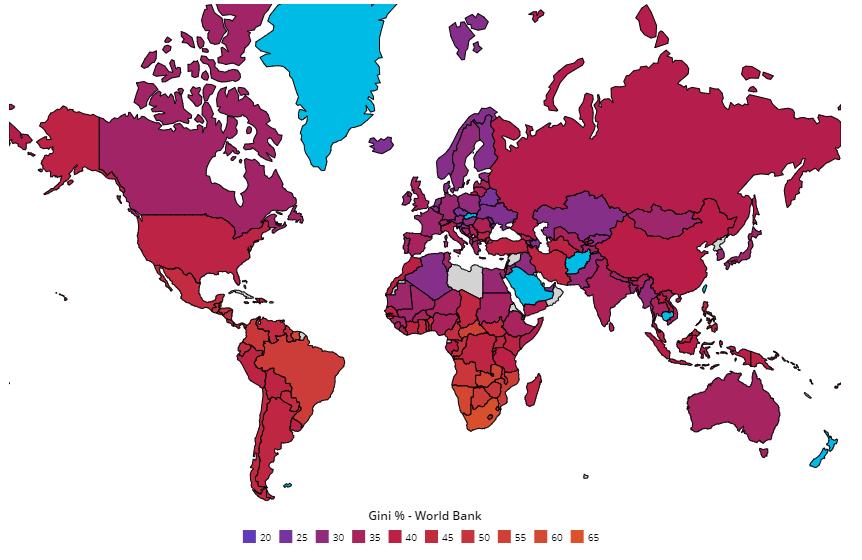
Source: World Bank Database (2022)
Figure 2 demonstrates the relationship between the top one percent’s share of the total wealth and the United States Gini Coefficient. From 1990-2019 the United States top one percent has seen an increase in their total share by 27.92 percent, and the Gini coefficient has seen an increase of 9.21 percent. This demonstrates that there is a positive correlation between the two, so as the top one percent’s share total share of the wealth increases so too will the Gini Coefficient within the United States.
Figure 1: Gini Coefficient by Country
27
Source: Federal Reserve Economic Data
Figure 3 shows how income inequality is distributed across the United States. The five states with the highest level of income inequality are New York, Connecticut, Louisiana, California, and Florida. The five states with the lowest level of income inequality are Alaska, Utah, Wyoming, New Hampshire, and Hawaii.
Source: United States Census Bureau (2021)
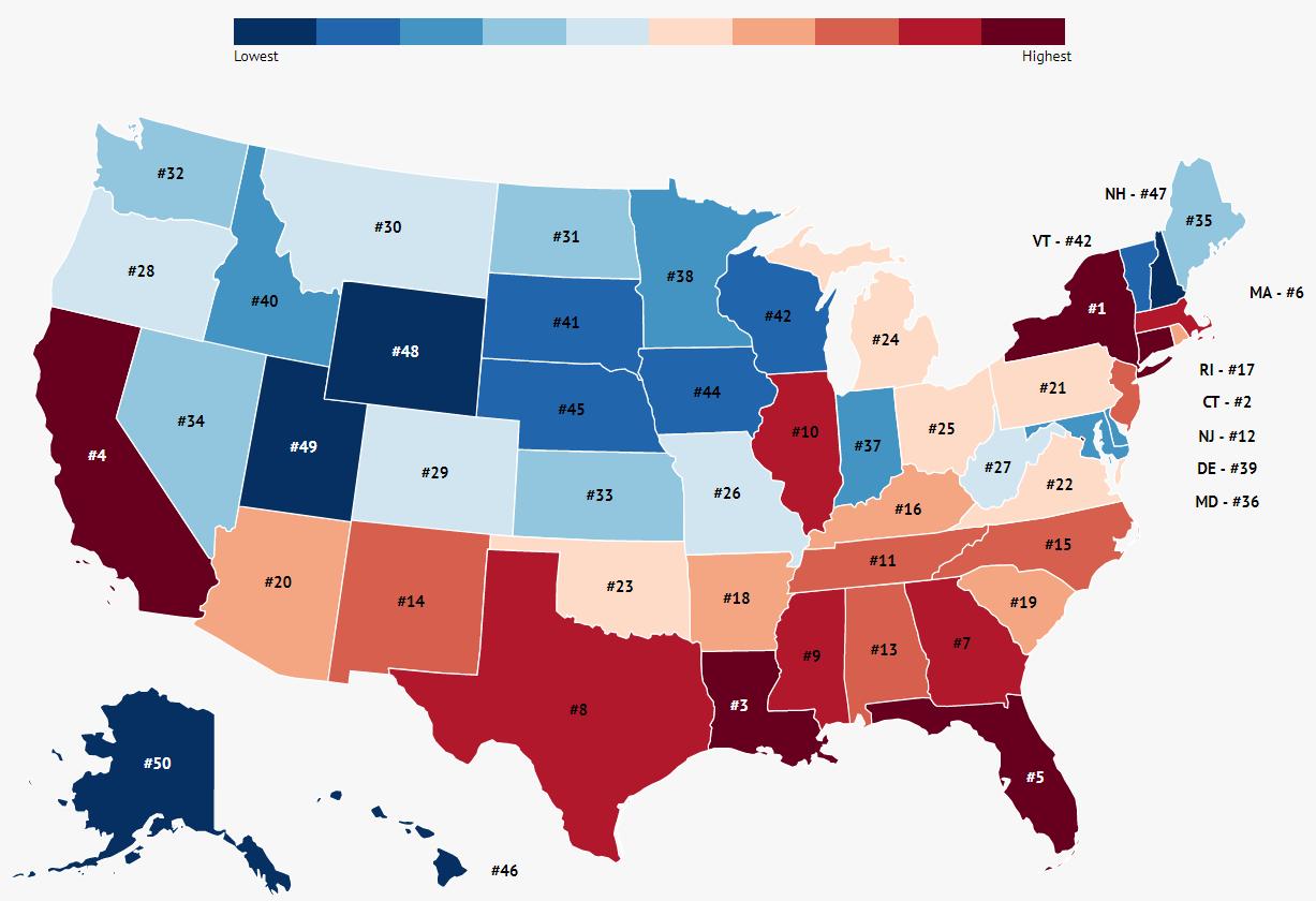 Figure 2: Top 1% Share of Wealth vs. Gini Coefficient
Figure 3: Inequality Distribution Across the United States
Figure 2: Top 1% Share of Wealth vs. Gini Coefficient
Figure 3: Inequality Distribution Across the United States
0 5 10 15 20 25 30 35 40 45
28
Top 1% Gini
Figure 4 shows real median household income when observed through the demographics of race, gender, age, and educational attainment. Race broken up white, and nonwhite. Gender is broken up using the two rudimentary genders of male and female. Age is broken up into three groups, being 15-34, 35-64, and 65 and older. And educational attainment is broken into four groups that include: no high school diploma, high school diploma but no college, some college, and bachelor’s degree or higher. The real median household income was adjusted for using 2020 CPI-U-Rs Dollars (Consumer Price Index Retroactive Series), and it utilizes current methods to present an estimate for all Urban Consumers (CPI-U) (U.S. Bureau of Labor Statistics). The three most affected groups from this figure are those without a high school diploma, those 65 years old or older, and women. It can also be observed that there is a significant variance between the real median household income of white individuals and nonwhite individuals.
4: Real Median Household Income vs. Demographics
Figure
0 20000 40000 60000 80000 100000 120000 2000 2001 2002 2003 2004 2005 2006 2007 2008 2009 2010 2011 2012 2013 2014 2015 2016 2017 2018 2019 U.S white nonwhite male fem edu1 edu2 edu3 edu4 age1 age2 age3 29
Source: United States Census Bureau Historical Income Tables (2019)
3.0 Literature Review
Who is it that suffers from income inequality? According to Alaya et al (2001) in a study done on OECD countries, those who are unemployed are the group most susceptible to the effects of income inequality. It was in this same study that it was also noted that unemployment is also responsible for inflating the effects of income inequality because in most cases those who are unemployed are poorer than those with jobs who hail from a wealthier background and have received a higher level of education. This point is expanded upon by Fuceri and Ostry (2019). In their study it was explained that demographics, unemployment, level of development and trade integration were some of the key drivers of income inequality. Paweenawat and McNown (2014), also discussed the effect of demographics while saying that gender differences of the head of the household, as well as differences in the composition of the household are significantly related to income inequality.
The study conducted by Rubin and Segal (2015), brings in the determinant of economic growth as it relates to income inequality. Through this it is discussed that according to the wealth hypothesis, if there is even the slightest increase in economic growth it will elicit a positive multiplier effect on the value of labor income, GDP per capita, and general wealth. All of this reduces the levels of income inequality present in a community. This is why the unit utilized for economic growth in this study is GDP per capita. Relating to economic growth trade openness also enhances economic growth (Balassa 1978). This trend is noted because trade openness allots local firms the opportunity to easily compete in international markets which has the ability to boost their expansion capacity and create employment. Inversely it was also noted by Kaplan and Rauh (2010), that economic growth can also be a driving factor for income inequality as it can cause more sensitivity to wealth than labor income. Additionally, Richmond and Triplett (2017) also noted that information and communication technology could potentially exacerbate income inequality. This was equated to the differences that ICT creates in the access to skills as not all socioeconomic classes have equal opportunities. On the opposite side of economic growth is the presence of poverty in an economy. Within the United States rural communities demonstrated a 2.4% higher rate of poverty than those of urban communities (USDA 2017). This was expanded upon by Akin-Olagunju and Omonona (2013) in their study of the households of Ibadan in the
30
Oyo State. Here it was revealed that there was a high presence of income inequality among rural households.
One of the most notable determinants that had a positive effect on real median household income was the presence of human capital development. The rationale behind this is described in Becker and Chiswick (1966) who mention hat high human capital development reduces the levels of income inequality at workplace and society in general. Education enhances the skills and competencies of individuals as well as their productivity. So, as it stands, those with a higher educational attainment have an increase’s chance of making more money, as their human capital is raised.
As it was stated before, those who are unemployed, are directly associated with an individual who has less money. But according to Jacoby (2000), as infrastructure development increases, so too do the benefits and opportunities present to the poor, thus making them more connected to economic activities. This is disputed by Tsaurai and Nyoka (2019) however. In their literature they discuss the possibility that infrastructure development can demonstrate negative effects on the poor. Resources that has the potential to boost labor income for citizens through small loan provisions are now being diverted towards long term infrastructure development. Another, determinant that was also noted to have the potential to negatively affect lower socioeconomic classes is financial development. Dhrifi (2013) discusses that as financial development increases it also increases the income inequality gap because the rich are able to become richer due to their ability to access credit. This ability allows them to invest in income generating projects.
4.0 Data and Empirical Methodology
4.1
Data
This project draws data from the United States Census Bureau, U.S. Bureau of Labor Statistics, U.S. Bureau of Economic Analysis, and Federal Reserve Economic Data (Fred). This data encompasses all fifty states from 2008-2019 and is utilized through panel data analysis. Summary Statistics for the data are provided in table 1.
31
Table 1: Summary Statistics
4.2 Pre-estimation Diagnosis
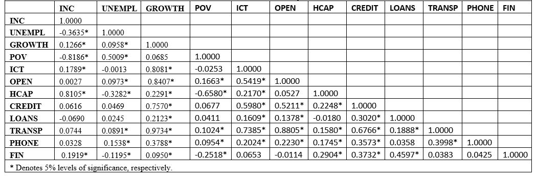
The Pearson Correlation method is the pre-estimation diagnosis that is covered under this subsection. According to table 2, the variables with were found to have a meaningful relationship with real median household income include unemployment, economic growth, poverty, information and communication technology, human capital, and finance. These results are backed says these variables are key determinants of income inequality. Trade openness, credit, transportation, and phone were all found to positively effect real median household income, although their results were insignificant. Loans were also insignificant, but they negatively impacted real median household income.
Variable Observation Mean Std. Dev. Min Max INC 600.00 62009.92 10262.62 35992.00 96765.00 UNEMPL 600.00 5.95 2.29 2.10 13.70 GROWTH 600.00 343435.70 429199.70 25999.25 3052645.00 POV 600.00 12.94 3.42 3.70 23.10 ICT 600.00 3083.25 9169.87 23.00 113659.90 OPEN 600.00 2337.21 3581.69 37.82 27371.12 HCAP 600.00 29.27 5.23 17.10 45.00 CREDIT 600.00 10607.75 20107.34 69.34 174053.30 LOANS 600.00 151000000.00 291000000.00 1565802.00 1640000000.00 TRANSP 600.00 16227.57 18389.72 1069.10 129829.40 PHONE 600.00 0.02 0.01 0.00 0.06 FIN 600.00 0.07 0.05 0.00 0.32
32
Table 2: Correlation Analysis
4.3 Empirical Model
The general model that this study is derived from is as follows:
Publicly available data for the fifty states excludes INEQ, ICT, HCAP, FDI, INFR, and FIN as they are defined by the first model, so the variables had to be adjusted accordingly to accurately represent this study. To this model we have added POV, CREDIT, LOANS, TRANSP, AND PHONE. The rationale behind adding poverty was to introduce an alternative perspective to economic growth. This perspective was discussed, but not included in Tsaurai (2020). The rationale behind the other four were to cover the variables that were not able to be included as much as possible in order to achieve comparable results. The reason that there is more than the base model is because the original variable encompassed a broader range of information then the data accessible for the fifty states, so additional data needed to be utilized.
The model utilized in this study can written as follows:
33
Independent Variables
There are eleven independent variables within this model, each possessing an individual relationship to the dependent variable of real median household income. Their data, description, expected sign, and what they capture are provided by appendix A and B. The variables, descriptions, and proxies that were not included in this study and used by the model this study is based on are provided by appendix C.
5.0 Empirical Results
5.1 Hausman Test
As it is demonstrated in the table 3, a Hausman test was conducted on the data that included the fixed effects test, the random effects test, and the pooled ordinary least squares test. It was determined that at a significance level of 5% the best test to explain the empirical model is the fixed effects test because the prob>chi value of .0232 was under .05.
34
Table 3: Hausman Test
a - Coefficients - a
(b) (B) (b-B) sqrt(diag(V_b-V_B))
b = Consistent under H0 and Ha; obtained from xtreg. B = Inconsistent under Ha, efficient under H0; obtained from xtreg.
Test of H0: Difference in coefficients not systematic
chi2(5) = (b-B)'[(V_b-V_B)^(-1)](b-B)
w = 13.02
iProb > chi2 = 0.0232
5.2 Regression Analysis
In table 4 the two variables of POV and HCAP were both significant at 1%. As educational attainment is a key factor in determining socioeconomic status, the results are consistent with Akin-Olagunju and Omonono (2013). Together they noted that rural households, which are more prone to poverty (USDA 2017), have high levels of income inequality, and that education reduced income inequality. Economic growth, trade openness, and phone were all significant at 5%, but trade openness significantly negatively impacted real median household income. This is backed up by Rubin and Segal (2015) and Kaplan and Rauh (2010). In there writings they state that a small increase in economic growth has got a positive multiplier effect on the value of labor income, GDP per capita, and the general wealth levels of the community. Economic growth and trade openness can also increase income inequality if it causes more
Fixed Random Difference Std. err. UNEMPL -13.91803 -10.45544 -3.462586 55.24206 GROWTH 0.0173576 0.010024 0.0073335 0.0066181 POV -1151.419 -1235.965 84.54663 30.71191 ICT -0.0353216 0.0053596 -0.0406812 0.0385111 OPEN -0.5809396 -0.2346341 -0.3463055 0.1394739 HCAP 1096.071 1050.355 45.71601 91.01297 CREDIT -0.0444673 -0.0423781 -0.0020891 0.0219339 LOANS 1.76E-06 8.90E-07 8.73E-07 8.30E-07 TRANSP -0.2265371 -0.1572582 -0.0692789 0.0798912 PHONE 91259.2 46705.1 44554.11 25053.79 FIN -16508.28 -14032.58 -2475.706 13811.6
35
sensitivity to wealth than labor income, meaning if only a small portion of the population are benefiting. Phone is supported by Jacob (2000) who claims infrastructure development benefits the previously disadvantaged and the poor as they can now be able to easily gain access to productive opportunities and more readily connect to economic activities. This is also why transportation only significant at 10% because the poor can now enjoy low transportation and production costs through easily accessing better road infrastructure. It also makes sense that their significance is lower because as Tsaurai and Nyoka (2019) state, resources that could have been used to boost small loans would now have to be diverted towards these long-term infrastructure projects.
6.0 Conclusion
This project’s main objective was to explore the determinants of income inequality using real median household income. It accomplishes this thoroughly the utilization of time-series data in the analysis of the Gini coefficient, the top one percent’s share of the wealth, and how the real median household income compares to varying demographics. It also accomplishes this through the use of a panel data analysis with a fixed effects regression, and random effects regression,
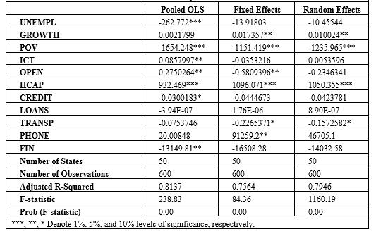 Table 4: Determinants of Income Inequality in the United States: Regression Analysis
36
and a pooled ordinary least squares regression. The results of these regressions were that economic growth and human capital had a significant positive effect on real median household income, and that unemployment and poverty rate had significant negative effects on real median household income. These results demonstrated the opposite of the results found in Tsaurai (2019). This fact makes sense though because their dependent variable was the Gini coefficient, which directly analyses income inequality, whereas my dependent variable was real median household income. So, anything that negatively impact income inequality would inadvertently positively impact median income. The policy implications of this study are that the United States should be urged to continue implementing policies that aid in economic growth, and combat unemployment and poverty. Six potential recommendations for this could be: to decrease the mortgage interest tax deduction, then use the additional revenue as credit for first-time homebuyers; to utilize automatic savings for retirement plans; to reduce dependence on student loans while supporting success in postsecondary education; to offer universal savings accounts for children; to reform asset tests for safety net programs, because they can act as barriers to saving among low-income families, and to provide subsidies similar to those linked to tax time, in order to promote emergency savings. The United States government should also work to increase the accessibility to upper-level educational systems because a high level of human capital development has been demonstrated to significantly effect the real median household income for the better.
37
Appendix A: Variable Description and Data Source
Acronym Description
INC Real median household income in state i at time t
UNEMPL Unemployment rate in state i at time t
GROWT
H Economic growth in state i at time t
POV Poverty rate in state i at time t
Data Source
U.S. Census Bureau Historical Data
Tables
Federal Reserve Economic Data
Federal Reserve Economic Data
Federal Reserve Economic Data
ICT Information and communication technology in state i at time t Federal Reserve Economic Data
OPEN Trade openness in state i at time t
HCAP Human capital development in state i at time t
CREDIT Credit in state i at time t
LOANS Loans in in state i at time t
TRANP Transportation expenditures in state i at time t
PHONE Telephone expenditures in state i at time t
FIN Internal financing in state i at time t
Federal Reserve Economic Data
Federal Reserve Economic Data
Federal Reserve Economic Data
Federal Reserve Economic Data
Federal Reserve Economic Data
Federal Reserve Economic Data
Federal Reserve Economic Data
38
Acronym
Appendix B: Variables and Expected Signs
UNEMPL Unemployment
GROWTH Economic growth
POV Poverty
ICT Information and communication technology
OPEN Trade Openness
HCAP Human capital development
CREDIT Credit
LOANS Loans
TRANSP Transportation expenditures
PHONE Telephone expenditures
Percentage of the total population involved in the labor force
Gross domestic product per capita
The percentage of the population living below the set standard of living -
Accessibility to the internet
Total of exports and imports (% of GDP)
Educational attainment (Bachelor’s degree or higher)
Monetary authorities-central bank, credit Intermediation, and related Services +
Total loans and leases, net of unearned income for commercial banks +
Gross domestic product: transportation and utilities
Broadcasting (except internet) and telecommunications
FIN Internal financing Finance and insurance
it Captures Expected Sign
Income Inequality
Variable Description What
INC Real median household income
-
+/-
+
+/-
+
+/-
+/-
+ 39
Appendix C: Excluded Variables
Acronym Proxy Used
ICT Individuals using the internet (% of the population)
HCAP Human capital development index
FDI
INFR
Net foreign direct investment (% of GDP)
Fixed telephone subscriptions (per one hundred people)
FIN
Market capitalization of listed domestic companies (% of GDP)
40
Work Cited
Afandi, A., Rantung, V.P., & Marashdeh, H. (2017). Determinants of income inequality. Economic Journal of Emerging Markets, 9(2), 159-171.
Akin-Olagunju, O.A., & Omonona, B.T. (2013). Determinants of income inequality among rural households of Ibadan, Oyo State, Nigeria. Nigerian Journal of Rural Sociology, 13(3), 2737.
Allison, C., Fleisje, E., Glevey, W., & Johannes, W.L. (2014). Trends and key drivers of income inequality. Working Paper, Marshal Society, Cambridge.
Arellano, M., & Bond, S. (1991). Some tests of specification for panel data: Monte Carlo evidence and an application to employment equations. The Review of Economic Studies, 58(2), 277-297.
Ayala, L. Carbonell, J.R., & Martinez, R. (2001). The impact of unemployment on inequality and poverty in OECD countries. Economics of Transition, 9(2), 417-447.
Azher, B.A. (1995). Rural savings: Their magnitude, determinants, and mobilization. Pakistan Development Review, 34(4), 779-786.
Bahmani-Oskooee, M., Hegerty, S.W., & Wilmeth, H. (2008). Short run and long run determinants of income inequality: Evidence from 16 countries. Journal of Post Keynesian Economics, 30(3), 463-484.
Balassa, B. (1978). Exports and economic growth: further evidence. Journal of Development Economics, 5(2), 181- 189.
“Bureau of Economic Analysis.” U.S. Bureau of Economic Analysis (BEA), https://www.bea.gov/.
Bureau, US Census. Census.gov, 6 May 2022, https://www.census.gov/.
Education, Income, and Ability - JSTOR. https://www.jstor.org/stable/pdf/1831252.pdf.
“Federal Reserve Economic Data: Fred: St. Louis Fed.” FRED, Federal Reserve Bank of St. Louis, https://fred.stlouisfed.org/.
Furceri, D., & Ostry, J.D. (2019). Robust determinants of income inequality. Oxford Review of Economic Policy, 35(3), 490-517.
Gini Coefficient by Country 2022, https://worldpopulationreview.com/country-rankings/ginicoefficient-by-country.
“ICYMI... Rural Families Headed by Single Adults Had Higher Poverty Rates than Urban Counterparts in 2017.” USDA ERS - Chart Detail, https://www.ers.usda.gov/dataproducts/chart-gallery/gallery/chart-detail/?chartId=95521.
International Monetary Fund. (2015). World Economic Outlook: Adjusting to Lower Commodity Prices. Washington (October). Retrieved from https://www.imf.org/en/Publications/WEO/Issues/2016/12/31/WorldEconomic-OutlookOctober-2015-Adjusting-to-Lower-Commodity-Prices-43229.
41
Jacoby, H. (2000). Access to rural markets and the benefits of rural roads. Economic Journal, 110(465), 713-737.
Kunofiwa Tsaurai. An Empirical Study of the Determinants of Income Inequality.
https://www.abacademies.org/articles/An-Empirical-Study-of-The-Determinants-ofIncome-Inequality-1528-2635-24-6-614.pdf.
Kaplan, S., & Rauh, J. (2010). Wall street and Main street: What contributes to the rise in the highest incomes?. Revised Financial Studies, 23, 1004-1050.
Levin, A., Lin, C.F., & Chu, C.S.J. (2002). Unit ro
Odhiambo, N.M. (2009). Finance-growth-poverty nexus in South Africa: A dynamic causality linkage. Journal of Socio-Economics, 38(2), 320-325.
Paweenawat, S.W., & McNown, R. (2014). The determinants of income inequality in Thailand: A synthetic cohort analysis. Journal of Asian Economics, 31, 10-21.
Public Disclosure Authorized Income Inequality and Poverty
https://www.researchgate.net/profile/NanakKakwani/publication/37883350_Income_inequality_and_poverty_methods_of_estimation_ and_policy_applications/links/57e0b63608aece48e9e20225/Income-inequality-andpoverty-methods-of-estimation-and-policy-applications.pdf?origin=publication_detail.
Richmond, K., & Triplett, R. (2017). ICT and income inequality: A cross-national perspective. International Journal of Applied Economics, 32(2), 1-20.
Rubin, A. & Segal, D. (2015). The effects of economic growth on income inequality in the US. Journal of Macroeconomics, 45, 258-273
Stead, R., & Wisniewsk M. (1996). Foundation quantitative methods for business. Prentice Hall. England. Stjepanovic, S. (2018). Income distribution determinants and inequality in Croatia. 34th International Scientific Conference on Economic and Social DevelopmentXVIII International Social Congress, Moscow, 18-19 October.
Stiglitz, J.E. (1993). The role of the state in financial markets. The World Bank Economic Review, 7(suppl_1), 19-52. Su, B., & Heshmati, A. (2013). Analysis of the determinants of income and income gap between urban and rural China. China Economic Policy Review, 2(1), 1-29.
Tridico, P. (2018). The determinants of income inequality in OECD countries. Cambridge Journal of Economics, 42(4), 1009-1042.
Tsaurai, K., & Nyoka, C. (2019). Financial development-income inequality nexus in South Eastern European countries: Does the relationship vary with the level of inflation? International Journal of Services, Economics and Management, 10(2), 110-125.
U.S. Bureau of Labor Statistics, U.S. Bureau of Labor Statistics, 6 May 2022, https://www.bls.gov/.
42
A Panel Data Analysis on Income Inequality on Life Expectancy in Asia
Julianna Flaccavento a
Abstract:
This paper aims to investigate the possibility of interdependence between income and life expectancy in countries across Asia. The study looks at the difference of life expectancies for men, women, and the two genders combined. We also looked at how health could have an impact on the model. We ran a fixed and random effect model on our panel data. We then ran the fixed and random effect model on the countries separated by income levels which we separated into low, middle, and high. The results show that the fixed effect was significant in Asia on both males and females and learned that the income separation does not have an impact at all.
JEL Classification: D33, E24, O15, P36
Keywords: Life Expectancy, Income Inequality.
a Department of Economics, Bryant University, 1150 Douglas Pike, Smithfield, RI02917. Phone: (845) 475-5075. Email: jflaccavento@bryant.edu.
43
1.0 INTRODUCTION
As life expectancies last longer, there has been a movement to live healthier and longer lives. With modern medicine we have increased the average life span from 52.5 years of age in 1960 to an average of 72 today. With the miracles of modern medicine and public health initiatives, we have helped ourselves extend lives so much that we may in fact be running out of innovations to extend life any further. The gains to further extend life expectancies are slowing worldwide (Ruggeri, 2018).
This study aims to enhance the understanding of income inequality on life expectancy. From a policy perspective, this analysis is important because it can help the government to implement policies to better balance out the income within each country across Asia. The relevance of this study is that it shows how an unequal spread of income can drastically affect how long people live. It affects the lifestyle that people live and can even hinder their health if they cannot afford proper healthcare. We also look to see how health expenditure within the different countries could impact life expectancies.
This paper was guided by three research objectives that differ from other studies: First, it investigates how income inequality can impact life expectancies in thirty-four countries across Asia using dynamic panel data; Second, it incorporates information on how different health expenditures within the countries can influence how long people live; Lastly, it looks at how incorporating an income separation can help to visualize how income inequality can impact life expectancies. There is very little empirical work in the literature concentrating on Asia as a country using a dynamic panel data model. This paper fills that void.
The rest of the paper is organized as follows: Section 2 gives a trend analysis Section 3 shows a brief literature review. Section 4 outlines the empirical model. Data and estimation methodology are discussed in section 4.2. Finally, section 5 presents and discusses the empirical results. This is followed by a conclusion in section 6.
2.0 LIFE EXPECTANCY TREND
Figure 1 shows the countries in Asia that we are studying and the life expectancy associated with each. The darker the country is shaded, the longer the life expectancy. This graph
44
also shows total life expectancy rather than a breakup of women and men. Figure 2 shows income per capita by country. A majority of the countries have income per capita under one hundred (shown as a percentage of growth). Any country over one hundred shows growth of adjusted net national income per capita as more than 100%. As for countries under 0, they show negative growth or a contraction in their economy.
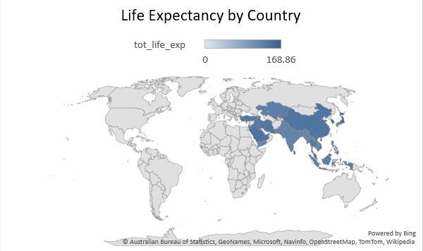 Figure 1: Life Expectancy by Country
45
Source: Author Contribution
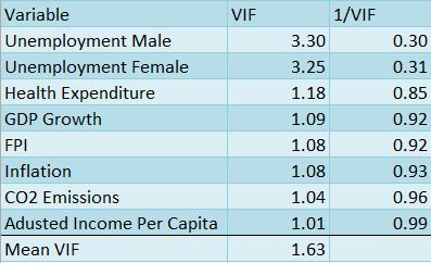
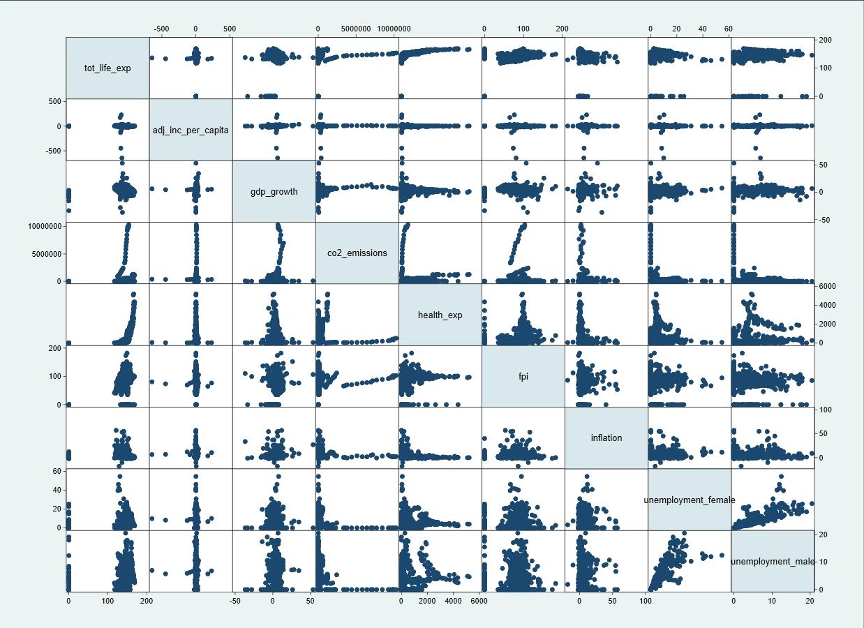
Figure 3 shows the correlation between variables run in the regression. As we can see below, we do not have any variables with multicollinearity or even a high correlation in general. The highest correlation we see is between the unemployment rate for men and women. Which is validated by the fact that if you aren’t a male, you are a female and vice versa. Figure 4 shows the variance inflation factor (VIF) which is a measure for testing multicollinearity. As a rule of thumb any variable with a VIF over 10 needs to be dealt with. This study did not have to deal with any of the consequences that are related to multicollinearity. The average VIF for the regression was 1.63 and the highest VIF was 3.30 which still is not high enough for us to act upon as it is well under our rule of thumb set at 10.
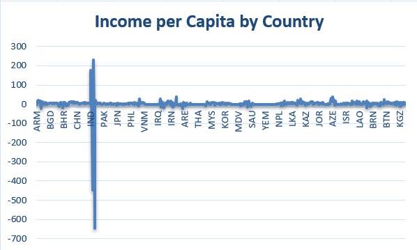
Figure 2: Income per Capita by Country
Source: Author Contribution
46
Figure 3: Correlation Matrix for Total Life Expectancy
Source: Author Contribution
Source: Author Contribution
Figure 4: Variance Inflation Factor
47
Source: Gisbert (2020)
Figure 6: Life Expectancy and Distributionally Adjusted Life Expectancy at Birth by Sex
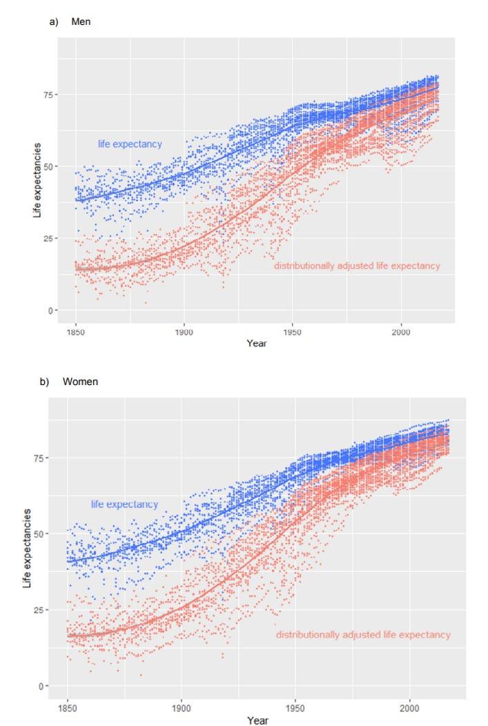
Source: Gisbert (2020)
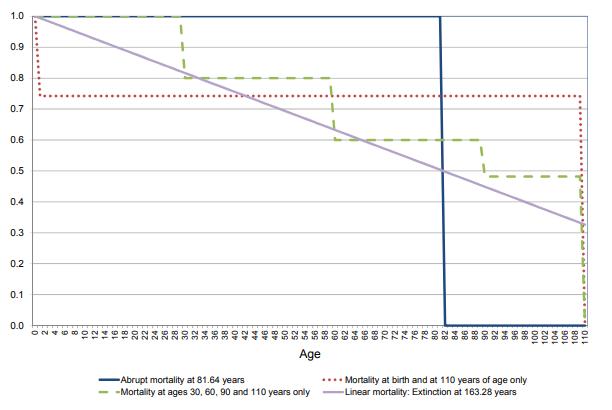 Figure 5: Alternative Survival Functions with the Same Life Expectancy at Birth
48
Figure 5 above shows different morality rates that we could experience. The solid blue line shows how everyone could live until they reach the age of 81.64 years old and then they die. In this case everyone has the same length of life. The dotted red line on the other hand, shows that at birth 25.78% of the population dies and the remaining 74.22% of the population survives until the age of 110. In this case mortality is concentrated at two points in the life of the generation, the beginning and the end. Nobody dies between these two extremes. In both the case of the solid blue line and the dashed red line, we see two extreme and unrealistic survival functions. In the case of the solid blue line, the survival function is a perfect rectangle. In the case of the dashed red line, a lottery determines whether you die just at the start of life or at the end of life. Since we only have two possible outcomes, the inequality in the distribution of life is at a peak. However, in both cases the population’s life expectancy is identical at 81.64 years although the two cases are extremely different. Now looking at the case of the dashed green line, every newborn survives until the age of 30 and then 20% of the population dies. Then the remaining 80% of the population lives until the age of 60 when another 20% of the population dies. Then the remaining 60% of the population survives until the age of 90 and then a further 11.8% of the initial population dies. The surviving 48.2% of the initial population then lives until the age of 110 when they all die abruptly. Lastly, we look at the solid purple line. According to this line, the newborns die at a linearly constant rate. The generation lives until the age of 163 years old although our graph only goes until the age of 110. All of these survival functions represent the same life expectancy but have very different implications for the age at death distribution (Gisbert, 2020).
Figure 6 above shows the life expectancies of men and women against inequity of life. In both cases we see the same convergence trend of the distributionally life expectancy approaching life expectancy over time. The reason behind the convergence is the strong negative correlation between the increases in life expectancy and the reduction in life length inequality. This reduction in inequality was strong during the mid-20th century and has slowed down considerably in recent years, essentially because infant mortality is so low in most developed countries that it is now difficult to reduce inequality in the length of life any further (Gisbert, 2020).
49
3.0 LITERATURE REVIEW
The impact of income inequality on life expectancy has been extensively studied and has led to a rise in a new front of empirical research. Gisbert (2020) studied how the impact of time across societies and the fact that populations have very different age structures can impact life expectancy while Hansen and Lonstrup (2011) looked at the correlation between schooling and life expectancy. Kriener et al. (2018) worked to compute the income gradient in period life expectancy that accounts for the mobility of income on life expectancy where Prus and Brown (2008) tested the income inequality population health hypothesis. Ali and Audi (2016) looked at the relationship between income distribution and health to see the impact that they might have on life expectancy. Regidor et al. (2003) looked at how both average income and measures of income inequality affect life expectancy.
Life expectancy at birth can summarize in a single number, the morality conditions of a given population (Gisbert, 2020). Since this single number can estimate morality conditions, it has become the most widely used indicator in international comparisons on development as well as the simplest summary measurement of population health for a community (Gisbert, 2020). Gisbert (2020) wanted to go beyond life expectancy by trying to introduce distributional aspects into a single life expectancy index that could be used more fluently over time and across countries. While Gisbert (2020) was trying to create an index that changed with each generation, Hansen and Lonstrup (2011) were looking at how an increasing life expectancy leads to more schooling. Their intuitive reasoning was, a longer expected working life, where the benefits of education are reaped, induces individuals to invest more into their human capital (Hansen & Lonstrup, 2011). These two economists saw a gap in the theoretical underlying concepts that didn’t include schooling when estimating life expectancy. The reasoning for the lack of including schooling into the life expectancy frameworks is due to the Ben-Porath mechanism which states that optimal schooling time increases if and only if lifetime working hours increase (Hansen & Lonstrup, 2011). Hansen and Lonstrup (2011) argue that the Ben-Porath mechanism relies heavily on the assumption of access to perfect financial markets. They relaxed this assumption to show that individuals’ optimal response to increased life expectancy may be
50
due to increase schooling time and at the same time decrease future working hours where the schooling investments pay off in terms of higher hourly wage (Hansen & Lonstrup, 2011). On the other hand, Kreiner et al. (2018) looked at how income mobility affects life expectancy. The relationship between income class and life expectancy within a society is important for evaluating equity and assessing the costs and benefits of public health and social security policies (Kreiner et al., 2018). It is well known that the morality rate is decreasing in income across individuals and this relationship is used to estimate the association between income and life expectancy (Kreiner et al., 2018). Using tax return data, it is expected that those in the top of the income distribution at age 40 can expect to live nearly 15 years longer than those in the bottom of the distribution. When they segregated period life expectancy by income class, the morality of older cohorts in the same income class is used to estimate future mobility which assumes that individuals stay in the same income classes over time (Kreiner et al., 2018). This is in contrast to evidence in economics and sociology documenting significant income mobility. The consequence of this is that estimates of the period life expectancy of the different income classes will in general not be equal to the observed average life length even when considering an unchanging society in which mortality and mobility rates are constant (Kreiner et al., 2018). Regidor et al. (2003) separated his population into males and females to see the effects of average income on life expectancy. They incorporated the Gini index and the Atkinson indices to see those effects as well.
The greater the dispersion of income within a country the lower its life expectancy which prompted Prus and Brown (2008) to study the health link on the topic at hand. They look at the psychosocial hypothesis which states that in addition to the importance of individual absolute income, relative income deprivation has a more direct effect on population health (Prus & Brown, 2008). Ali and Audi (2016) on the other hand look at how fair income distribution increases the health outcomes because it enables poor population to get a large share in profits and spend it on food and health cares. Environmental quality is an important factor which has a deep impact on human health of present and forthcoming generations. The way people value future is crucially affected by others moreover the present long life encourages people to become sympathetic to forthcoming generations (Prus & Brown, 2008).
51
4.0 DATA AND EMPIRICAL METHODOLOGY
4.1 Data
The study uses annual panel data from 2000 to 2020 for 35 countries in Asia. Data was obtained from the Bureau of Economic Analysis (BEA) website World Development Indicators. Summary statistics for the data are provided in Table 1.
4.2 Empirical Model
Following Ali and Audi (2016) this study was adapted and modified so we can run a fixed and random effect model. This study was modified to include multiple countries compared to the one country that Ali and Audi (2016) used so that we could run our panel data analysis regressions.
The ordinary least squares (OLS) model could be written as follows:
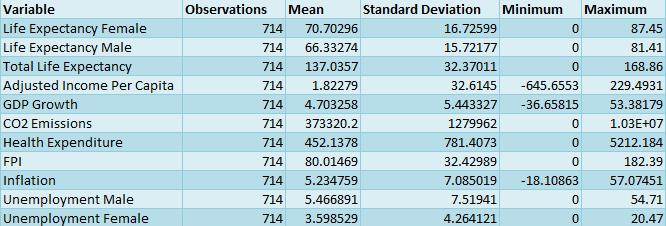 Table 1 Summary Statistics
���������������� ������������������������������������������������ = �������� + �������� �������������������������������� ������������������������ ������������ ������������������������ + �������� ������������ ������������������������ + �������� ������������ ������������������������������������ + �������� ������������������������ �������������������������������������������� + �������� ���������������� ���������������������������������������� �������������������� + �������� ������������������������������������ + �������� ���������������� ������������������������������������������������ + �������� ������������������������ ������������������������������������������������ + ���� (1) 52
���������������� ������������������������������������������������ is the expectancy at birth for males and females for people in country i at year t. ���������������� ������������������������������������������������ is used as an endogenous variable. It represents the life expectancy at birth that would prevail if patterns of mortality at the time of its birth were to stay the same throughout its life. We used life expectancy in three different ways. One set of regressions used life expectancy of males as the endogenous variable. Another set of regressions used life expectancy of females as the dependent variable. Lastly, the third set of regressions used total life expectancy as the endogenous variable. Independent variables consist of eight variables obtained from the World Development Indicator (WDI). Appendix A and B provide data source, acronyms, descriptions, expected signs, and justifications for using the variables. First, �������������������������������� ������������������������
represents income inequality in the host country (used as a proxy for the Gini coefficient). ������������ ��������������������ℎ is used to show the growth within the host country so we can see how much the country has improved over the years. ��������2
is used to show the environmental degradation in the countries while
�������������������� are used to show how much the country spends on healthcare and the availability of food within the region respectively. Our last three variables
are all used to represent economic misery. The combination of these three variables is also referred to as the misery index which is used to measure the degree of economic distress felt by everyday people. ���� represents the random disturbance within the model that could be present and ����0 represents some constant.
In this study we ran an Ordinary Least Squares (OLS) regression on life expectancy for males, females, and the two genders combined. After we interpreted these results, we ran a fixed (FE) and random (RE) effect regression on our empirical model. After we ran these tests, we had to perform a Hausman test to see which model was superior.
5.0 EMPIRICAL RESULTS
5.1 EMPIRICAL RESULTS FOR MALES
The purpose of this study is to find the possible interdependence of income inequality on life expectancy. The empirical estimation results are presented in Tables 2, 3, and 4.
The empirical estimation shows the negative relationship between CO2 emissions and
ℎ����������������ℎ �������������������������������������������� ������������ ����������������
������������������������������������, ���������������� ������������������������������������������������ , ������������ ������������������������ ������������������������������������������������
������������ ������������������������
������������������������������������
����������������������������������������
53
adjusted income per capita on life expectancy as well as the positive relationship between health expenditure and life expectancy. The fixed effect was the superior model for males, females, and the two genders combined when we tested the models under the Hausman test.
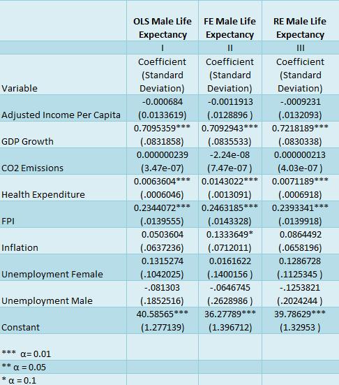
Table 2: Regression Results for Males
Note: *** , **, and * denotes significance at the 1%, 5%, and 10% respectively. Standard errors in parentheses
GDP growth, health expenditure, and FPI were all significant at the 1% level. The results under the fixed effect are in accordance with Ali and Audi (2016). After we ran the fixed effect, we saw that inflation became significant at the 10% level. CO2 emissions is only in accordance with Ali and Audi (2016) when we ran the fixed effect model as well
54
5.2 EMPIRICAL RESULTS FOR FEMALES
Table 3: Regression Results for Females
Note: *** , **, and * denotes significance at the 1%, 5%, and 10% respectively. Standard errors in parentheses
GDP growth, health expenditure, and FPI were all significant at the 1% level. The results under the fixed effect are in accordance with Ali and Audi (2016). After we ran the fixed effect, we saw that inflation became significant at the 5% level. Adjusted income per capita is only in accordance with Ali and Audi (2016) when we ran the fixed effect. CO2 emissions doesn’t have the sign we would expect when we ran OLS, fixed, or random effect.
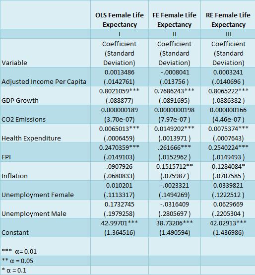
55
5.2 EMPIRICAL RESULTS FOR MALES AND FEMALES
Table 4: Regression Results for Males and Females
Note: *** , **, and * denotes significance at the 1%, 5%, and 10% respectively. Standard errors in parentheses
Our results for the two genders combined have an extra set of regressions compared to the men and women regressions and this is due to the fact that we also did an income separation based on GDP growth. We separated the countries into a low, middle, and high income. In the end, we couldn’t use the results from the regressions with the income separation. When we ran the Hausman test the results ended up showing that the data failed to meet the asymptotic assumptions. Instead, we had to change the Hausman test to only run on the regressions without the income separation. When we did this the fixed effect (without the income separation) was superior.
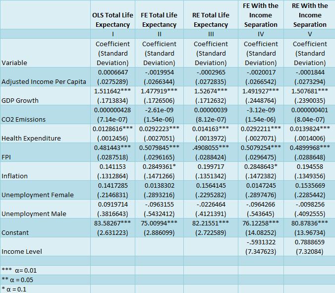
56
GDP growth, health expenditure, and FPI were all significant at the 1% level. The results under the fixed effect are in accordance with Ali and Audi (2016). After we ran the fixed effect, we saw that inflation became significant at the 10% level. CO2 emissions is only in accordance with Ali and Audi (2016) when we ran the fixed effect.
6.0 CONCLUSION
In summary, GDP growth, health expenditure, and FPI are all relevant factors when determining life expectancy. Inflation is only significant when running a fixed regression. The results in this paper imply that CO2 emissions and adjusted income per capita reduce life expectancy. This means that when there is a higher income gap, there is a lower life expectancy and same with CO2 emissions. Moreover, more health expenditure increases life expectancy. Economically, it is possible that separating the countries by income does not have an effect on life expectancy. It is also possible that unemployment also doesn’t affect life expectancy. However, if the assumption of time invariant is true, we will see each country having the same intercept year over year compared to time variant when it changes every year. Nevertheless, this paper shows that there is interdependence between income and life expectancy. Thus, analysis should consider the differences between income standings when trying to find life expectancy. To create a better model to estimate life expectancy, economists should also consider environmental degradation, health infrastructure, and availability of food. In addition, they should look at different factors of economic misery to see if other factors besides unemployment and inflation also have an impact on the model.
57
Appendix A: Variable Description and Data Source
Acronym Description
Life Expectancy Female
Life expectancy at birth indicates the number of years a newborn infant would live if prevailing patterns of mortality at the time of its birth were to stay the same throughout its life.
Data source
World Development Indicators (WDI)
Life Expectancy Male
Life expectancy at birth indicates the number of years a newborn infant would live if prevailing patterns of mortality at the time of its birth were to stay the same throughout its life.
World Development Indicators (WDI)
Total Life Expectancy
Adjusted Income Per Capita
GDP Growth
Calculated field based on the female and male life expectancy at birth.
Adjusted net national income is GNI minus consumption of fixed capital and natural resources depletion.
Annual percentage growth rate of GDP at market prices based on constant local currency. Aggregates are based on constant 2015 prices, expressed in U.S. dollars. GDP is the sum of gross value added by all resident producers in the economy plus any product taxes and minus any subsidies not included in the value of the products. It is calculated without making deductions for depreciation of fabricated assets or for depletion and degradation of natural resources.
Calculated
World Development Indicators (WDI)
World Development Indicators (WDI)
CO2 Emissions
Carbon dioxide emissions are those stemming from the burning of fossil fuels and the manufacture of cement. They include carbon dioxide produced during consumption of solid, liquid, and gas fuels and gas flaring.
World Development Indicators (WDI)
Health Expenditure
Current expenditures on health per capita in current US dollars. Estimates of current health expenditures include healthcare goods and services consumed during each year.
World Development Indicators (WDI)
58
FPI
Food production index (FPI) covers food crops that are considered edible and that contain nutrients. Coffee and tea are excluded because, although edible, they have no nutritive value.
World Development Indicators (WDI)
Inflation
Inflation as measured by the consumer price index reflects the annual percentage change in the cost to the average consumer of acquiring a basket of goods and services that may be fixed or changed at specified intervals, such as yearly. The Laspeyres formula is generally used.
Unemployment Female Unemployment refers to the share of the labor force that is without work but available for and seeking employment. Definitions of labor force and unemployment differ by country.
Unemployment Male Unemployment refers to the share of the labor force that is without work but available for and seeking employment. Definitions of labor force and unemployment differ by country.
World Development Indicators (WDI)
World Development Indicators (WDI)
World Development Indicators (WDI)
59
Adjusted Income Per Capita
Inflation
Appendix B- Variables and Expected Signs
Gross National Income minus consumption of fixed capital and natural resources depletion
Income inequality -
Health Expenditure
Inflation as measured by the consumer price index reflects the annual percentage change in the cost to the average consumer of acquiring a basket of goods and services that may be fixed or changed at specified intervals, such as yearly. The Laspeyres formula is generally used.
Current expenditures on health per capita in current US dollars. Estimates of current health expenditures include healthcare goods and services consumed during each year.
FPI Food production index (FPI) covers food crops that are considered edible and that contain nutrients. Coffee and tea are excluded because, although edible, they have no nutritive value.
Unemployment Male
Unemployment refers to the share of the labor force that is without work but available for and seeking employment. Definitions of labor force and unemployment differ by country.
Unemployment Female
Unemployment refers to the share of the labor force that is without work but available for and seeking employment. Definitions of labor force and unemployment differ by country.
GDP Growth
Annual percentage growth rate of GDP at market prices based on constant local currency. Aggregates are based on constant 2015 prices, expressed in U.S. dollars. GDP is the sum of gross value added by all resident producers in the economy plus any product taxes and minus any subsidies not included in the value of the products. It is calculated without making deductions for depreciation of fabricated assets or for depletion and degradation of natural resources.
Economic misery +/-
Health infrastructure +
Availability of food +
Economic misery +/-
Economic misery +/-
Economic growth +
Variable Description
it captures Expected sign
Acronym
What
60
CO2 Emissions
Carbon dioxide emissions are those stemming from the burning of fossil fuels and the manufacture of cement. They include carbon dioxide produced during consumption of solid, liquid, and gas fuels and gas flaring.
Environmental degradation _
61
BIBLIOGRAPHY
Ali, A., & Audi, M. (2016). The Impact of Income Inequality, Environmental Degradation and Globalization on Life Expectancy in Pakistan: An Empirical Analysis. Munich Personal RePEc Archive, 17.
Gisbert, F. J. (2020). Distributionally Adjusted Life Expectancy as a Life Table Function. Demographic Research , 38.
Hansen, C. W., & Lonstrup, L. (2011). Life Expectancy and Income: The Ben-Porath Mechanism Revisited. Discussion Papers on Business and Economics, 1-15.
Kreiner, C. T., Nielsen, T. H., & Serena, B. L. (2018). Role of Income Mobility for the Measurement of Inequality in Life Expectancy. PNAS, 1-6.
Prus, S. G., & Brown, R. L. (2008). Social and Economic Dimensions of an Aging Population Age-Specific Income Inequality and Life Expectancy: New Evidence. SEDAP, 1-35.
Regidor, E., Calle, E. M., Navarro, P., & Dominguez, V. (2003). Trends in the Association Between Average Income, Poverty, and Income Inequality and Life Expectancy in Spain. Social Science and Medicine, 1-11.
Ruggeri, A. (2018, October 2). Do we really live longer than our ancestors? Retrieved from 100 Year Life: https://www.bbc.com/future/article/20181002-how-long-did-ancient-peoplelive-life-span-versus-longevity
62
The School-to-Prison Pipeline: A Panel Data Analysis
By: Samuel J. Guider
Abstract: The objective of this paper is to analyze the potential affect public-school funding has on juvenile incarceration rates in the United States using a panel series data set from 2000 until 2020. The United States has the highest per capita incarceration rates among 114 other members of the Organization of Economic Co-operation and Development (OECD), with 639 individuals for every 100,000 are incarcerated in the United States. This papers aims to use explanatory variables like race (black and white), sex, age, arrests, educational attainment, and rates of school attendance to further help in answering if an increase in public spending on education will have an adverse effect on the rate of incarceration across the United States prison system.
JEL Classification: A22, C40, Z00

Keywords: school-to-prison pipeline, juvenile, incarceration rates, public-school, funding, United States, mass incarceration, zero tolerance policies.
a Department of Economics, Bryant University, 1150 Douglas Pike, Smithfield, RI, 02917.
Email: samuel.guider22@gmail.com
63
1. Introduction
The United States has the highest rate of incarceration across all aspects of its population (both Juvenile and adult incarceration rates). According to the Sentencing Project and a study done by PEW Research approximately 639 individuals for every 100,000 are incarcerated in the United States, the highest for any country (Gramlich 2021). El Salvador falls right behind the US with a ratio of 572 for every 100,000. Over the past few decades, the rate of incarceration has increased 500% since 1970 and there has been a growing convergence between schools and legal systems
(Sentencing Project 2022). The school-to-prison pipeline refers to a growing pattern of tracking students out of educational institutions, primarily via "zero tolerance" policies, both directly and indirectly, into the juvenile and adult criminal justice systems. A growing critique of these policies has led to calls for reformation in the prison industrial complex as well as other alternatives. A result of zero tolerance policy such as the suspension and/or expulsion of a student with no means of alternative or rehabilitative form of punishment i.e., school community service whilst keeping the student enrolled in school curriculum. Furthermore, this study analyzed the relationship a lack of school funding can have on youth incarceration, specifically minority communities and people of color, as well as the relationship between school attendance and a student's likelihood of being incarcerated.
2. Incarceration Rates
A regressive trend has emerged in the juvenile justice system over the last 40 years. The juvenile justice system shifted rather distinctly from its original rehabilitative and reform goals. These non-rehabilitative policies like juveniles being tried as adults and zero tolerance policies disproportionately and systemically affect people of color. Furthermore, these policies only
64
perpetuate racial inequity more importantly inequity amongst juvenile populations. Over 2.1 million persons are in state or federal prisons and jails, at a rate of 639 for every 100,000 individuals (Gramlich 2021). Although this is historically the lowest incarceration rate of the United States since 1995, much of this can be attributed to the COVID-19 Pandemic where prisons reached on average a 90% rate of capacity. This is the result of prisons admitting fewer inmates, not releasing more (Prison Policy Initiative 2022), and not an accurate depiction of incarceration. In other words, while it may be true to say we can observe a reduction in the rate of crime by in large, we are still seeing the same rate for incarceration across all groups i.e., race, gender, physical/mental disability, age, etc.
3. Trends
Figure 1A looks at the difference in the amount of costs per inmate and per student. Using the data collected from my research indicates a strong disparity between the cost per inmate vs. the cost per student. The highest for both metrics was New York. New York on average spent about $70,000 per inmate whilst simultaneously only spending approximately $25,000 on a single student. Local, state, and Federal governments combined, spend an average of $37,060 a year to keep a single inmate behind bars (See Figure 1). Furthermore, an average of $14,498 is spent on a child in the United States education system (see figure 1)
Figure 1B is similar to 1A, however, it gives a more comprehensive breakdown of k-12 public spending per student. The federal government provides 7.0% of funding for K-12 education, leaving an overwhelming reliance at the state and local levels to fund K-12 public education. The national average for spending on K-12 schools is 3.1% of the Gross Domestic Product (GDP).
65
Figure 1A: Cost per inmate vs per student Figure 1B: Public K-12 Spending Per Student
Figure 2 is a graph from the U.S. Department of Education. It recorded rates of suspensions by race from 1973 through 2006. It is worth reminding the rate of incarceration increased over 500% since 1970. Figure 2 shows the disproportionate rate of suspension for young black students between 1973-2006. It says that for ever 100 black students, roughly 15 are expected to be suspended every year. Following behind them are Native Americans with a suspension rate of 10 out of every 100, 7 for Latino/a/x, 5 for Whites, and 3 for every 100 Asian students.
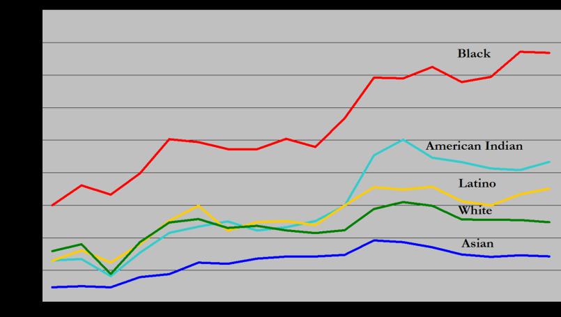
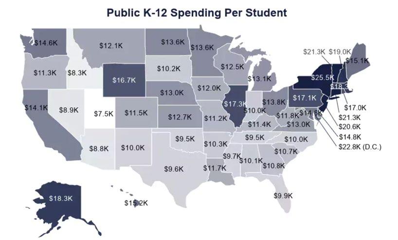
Michelle Alexander, Author of A New Jim Crow, discusses extensively in her book the redesigning of the American Prison System as such: “In the era of colorblindness, it is no longer socially permissible to use race, explicitly, as a justification for discrimination, exclusion, and
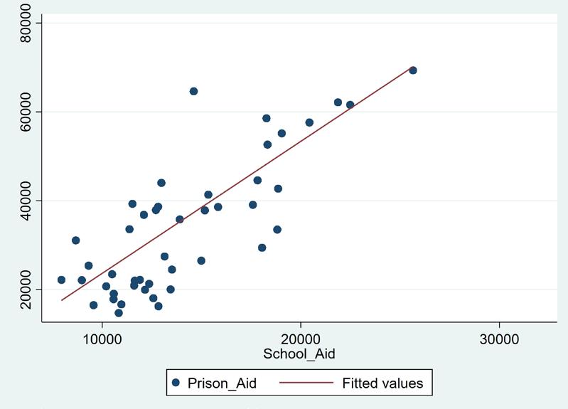 Figure 2: Suspension Rates by Race, 1973-2006
66
social contempt. So, we don’t. Rather than rely on race, we use our criminal justice system to label people of color ‘criminals’ and then engage in all the practices we supposedly left behind… We have not ended racial caste in America; we have merely redesigned it”.
Figures from past research and studies suggest a disproportionate level of arrest across minority groups when compared to those who identify as White. In the United States today, youth of color in America, predominantly young black boys account for 2/3 of those who are imprisoned. A shocking statistic reveals that 1 in 3 black men born after 2001 will be behind bars at some point in their lives. Where 1 in 111 white women will experience imprisonment in their life, that figure drops to 1 in 45 for Latinx women and 1 in 11 for black women. Furthermore 1 in 7 people in prison are serving life with parole, life without parole, or serving 50 years or more (Sentencing Project 2022).
4. Literature Review
Heitzeg (2009) discusses “zero-tolerance” policy and how it is these policies that perpetuate the “pipeline” towards incarceration. According to Heitzeg the school-to-prison pipeline has emerged over the propagation of youth violence and the mass incarceration that characterizes the legal systems. Furthermore, Heitzeg suggests while the school-to-prison pipeline is perpetuated by a number of trends, it is most directly attributed to the expansion and implementation of zero tolerance policies. These policies have no measurable impact on school safety but are associated with a number of negative effects' that are racially disproportionate, increased suspensions and expulsions, elevated risk of dropout rates, and multiple legal issues related to due process and mass incarceration.
67
Ellison et. al. (2017) analyzed the potential relationship between state fiscal effect towards education and if that decreased the rate of incarceration across juveniles ages 12-17. Ellison et all concludes the chance of detainment increases 3.5 times when adolescents drop out of high school. These findings further enhance the importance of investment in education. This paper had findings that support my hypothesis that increasing state fiscal effort for education leads to a decrease in juvenile incarceration expenses. Further analysis looked at the cost of juvenile incarceration vs. education. Similarly, my data found that the cost for incarceration was significantly higher than the cost per year to keep a juvenile in school. They concluded it costs approximately $148,000 to keep a juvenile incarcerated compared to just under $12,000 per year per juvenile to keep them enrolled in school. I used much of Ellison et. al.’s variables to assist in supporting my hypothesis that an increase in public education spending would decrease the rate of incarceration for juveniles across the United States. In conclusion, fiscal spending towards education seems to have a positive relationship and a negative relationship with incarceration rates.
Vernikoff (2018) looked at the relationship between students and youth who received special education services (students with learning and cognitive disabilities) and incarceration in the State of New York. Although this research had a dependent variable that differed from the scope of my research question, Vernikoffs conclusions further solidified the deeply rooted disproportionate levels of arrest across multiple minority groups. In addition, their research offers the implications of policy towards minority youth and how gaining a better understanding of how different factors, policy, and experiences can correlate with and effect the probability of arrest across juveniles.
68
5. Data and Empirical Methodology
5.1 Data
This study looked at data from the IPUMS US Census Data as well as the National Center for Educational Statistics and the Prison Policy Initiative. The dependent variable Incarceration is a proxy as it pertains to types of group quarters, one being Correctional Institutions which my research. 5 states were omitted due to lack of data concerning the cost per inmate as well as the District of Columbia and Puerto Rico. Appendix A provides the variable, variable description, its expected sign to the dependent variable, as well as a rationale behind why previous literature, including my own estimations and conclusions behind the relationship of my dependent and independent variables.
5.2 Empirical Methodology
The formula for the model can be written as follows:
Incarceration = ����0 + ����1 (prison_aid) + ����2(school_aid) + ����3 (sex) + ����4 (White) + ����5 (Black) + ����6 (Attendance) + ����7 (Education) + e
The dependent variable, incarceration is a proxy as it considers those who currently reside in Group Quarters. These group quarters consist of military, elderly, mental, and prisons. For the sake of this research, I was only concerned with Group Quarters of those in correctional facilities. More specifically, this model looks at individuals between 12 and 17 who would be considered juveniles that have been or are currently in correctional facilities across the United States.
69
There are seven other independent variables which derive from a number of sources, most of which were obtained through the Integrated Public Use Microdata Series (IPUMS). IPUMS is the world's largest individual-level population database consisting of microdata series across the United States The Education Data Initiative was also used in gathering data on the public education spending per student across 45 states.
The variable prison_aid is the first independent variable concerned with the amount in USD going to each incarcerated individual. School_aid looked conversely at the amount in USD that goes towards students. These two variables were extremely important throughout the majority of my research. While every state had a significantly higher cost per inmate than it did per student, the numbers suggest States with a motivation towards education vs those who may not. The variables sex, white, black, and attendance were all dummy variables. Where the variable sex identified male and female in my model, white and black identified individuals who identify as either black or white. Attendance was concerned with whether an individual was attending school regularly or not. Lastly, the variable education took the range of level of education received by those ages 12-17 and was used to identify any discrepancies between educational attainment and incarceration.
6. Empirical Results
The overall aim of this paper is to determine whether or not there is a significance between an increasing amount of school aid and a decrease in the rate of incarceration across students and youth. This model attempted to use the Hausman Effect, however, due to extremely high levels of homoscedasticity as seen from Table 3, the results could not be run across fixed, random, and OLS. My hypothesis that an increase in the allocation of spending towards public schools will result in the decreasing rate of incarceration with a significance at the 5% level. My model also
70
suggested an increase in the rate of students who attend school would significantly drop the incarceration rate. The estimation of my regression result is below:
Incarceration = -2.73e-04 + 4.23e-10(prison_aid) - 3.41e-09(school_aid) + 2.36e-07(sex) - 5.21e06(White) + 2.23e-05(Black) - 7.77e-05(Attendance) - .000078(Education) + e
The results from the regression can be found in Appendix B. A quiet reg was also run as well as a variance inflation indicator (VIF). My regression had a VIF of 2.31 which indicates that my model is considered to be low-moderately correlated. Table I is a break down of my main model, Model 2 as well as two other regressions concerned with other factors. Model 1 looked at the relationship prison and school aid had on incarceration. Model 3 was concerned with the effect that a lack of attendance can have on black youth across the 45 states observed in my analysis. Table 2 is a simple regression of the summary statistics of my main regression Model
2. Three of my variables sex, education, and school_aid was significant at the 5% level
7. Implications & Conclusion
7.1 Implications
A business will always maximize its profits; for-profit prisons are no exception. The only notable difference is that a prisons “good” or “service” is locking people up. By shifting from incarceration and instead, towards rehabilitation we would see a decrease in the number of individuals getting arrested and staying in prison. Conversely, moving away from for-profit prisons has the potential to eliminate the incentive for these “businesses” to maximize their profits be ensuring that have an above 90% capacity for individuals in prison.
7.2 Conclusion
71
The limited availability of data, and literature reviews with econometric models identifying the significance of the issue. I believe to have contributed to my overall regressions and findings. In hindsight, using a proxy as my dependent variable had the potential to significantly skew my data and I believe that using a more specific variable like the number of arrests per individual, my data would be more heteroskedastic, thereby decreasing the weight of the tailed distribution and increasing the level of symmetry throughout the model. School_aid was statistically significant at the 5% level suggesting that an increase in public funding for K-12 schools would decrease the rate of incarceration. Delivering a concise conclusion as to the true effectiveness of my model and empirical analysis is challenging due to a number of missing/unavailable data, the integration of one or more proxies into my model had the probability of skewing my results in either way, and indicators suggesting high homoskedasticity in the model which indicates disproportionate levels of collinearity. In an attempt to try running my regression again, fixing the parameters I have outlined I believe would have further strengthened my econometric model as well as my findings. By doing so, I could have had a more efficient run of the Hausman Test.
72
Variables Model 1 Model 2 Model 3 Sex 4.23e-10 (.041)** Prison_Aid 4.03e-07 (-.047)* -0.000078 (-.1.92) Education -3.41e-09 (-.032)** School_Aid -1.19 (-.11)** -7.77e-05 (-0.046)** -5.98e-07 (-0.031)** Age Attendance -5.21e-06 (-10.05) White -2.23e-05 (-.125) -2.018e-05 (1.098) Black 2.36e-07 (10.06) Constant -1.51e-05 (-10.21) 0.000018 (9.13)*
Table I
Variable Observation Mean Std. Dev. Min Max Incarceration 1,400,213 .0116629 .1073634 0 1 Prison_Aid 1,400,213 37060.44 17867.4 14740 69355 Education 1,400,213 2.92709 1.193777 0 8 School_Aid 1,400,213 14498.53 4396.276 7416 25651 White 1,400,213 .7649902 .424005 0 1 Black 1,400,213 .1347 .3414029 0 1 Sex 1,400,213 .4849004 .499772 0 1 Age 1,400,213 14.52978 1.707265 12 17 Attendance 1,400,213 .9734675 .1607127 0 1 73
Table 2
Table 3 Cameron & Trivedi's decomposition of IMtest chi2 df P-value Heteroskedasticity 1252.77 50 .0501** Skewness 494.49 9 .0000 Kurtosis 640.32 1 .0000 Total 2387.58 60 .0000 Table 4 Incarcera tion Sex Prison_ Aid Education School_Aid Attend ance Black White Age Incarceration 1.0000 Sex -0.0043 1.0000 Prison_Aid 0.0043 0.0001 1.0000 Education 0.0126 0.0227 0.0442 1.0000 School_Aid -0.0046 0.0008 0.7206 0.0273 1.0000 Attendance -0.0555 0.0094 0.0150 -.0446 0.0088 1.0000 White -0.05170.0027 -0.0696 -.0087 -0.0223 0.0166 1.0000 Black 0.0739 .0000 -0.0719 -.0076 -0.0108 -.0160 0.6126 1.0000 Age 0.0603 -.0045 0.0041 0.8142 0.0039 -.0680 -.0063 0.0058 1.000 0 74
Appendix A: Variables and Expected Signs
Incarceration
Proxy used to analyze the number of incarcerated individuals who are residing in “Group Quarters/institutions
n/a Dependent variable
Sex
Dummy variable identifying males as 0 and female individuals as 1 -
With men being more likely to be incarcerated, the expected relationship between sex and the dependent variable is negative
prison_aid
The amount of funding allocated to each prisoner at the State and Federal level +
An increase in the cost per inmate will only increase the number of incarcerated
Education
The level of education each individual student has attained
Increasing the education rate of juveniles will decrease the likelihood of them being incarcerated, which would have a negative impact on my dependent variable
school_aid
The amount per child/student the state/federal funding allocates to its education spending
Increasing the amount of pub school funding dramatically deceases the number of incarcerated juveniles
Attendance
Variable measuring the child still attends school or if they are no longer attending
An increase in the number of kids not attending school/classes would have a negative effect on the number of incarcerated juveniles
Black
Individuals who identify as black have a 1, all others are replaced with a 0
With the advancement of education into areas like the criminal justice system, we can expect such a system to maintain systemically racist institutions and as a result, individuals who identify as black will be more likely to end up in prison
White Individuals who identify as white have a 1, all others are replaced with 0
Age
This variable looks at kids ages 1217 as the study is aimed at identifying juvenile incarceration
As a result of systemic racism and inequality within the justice system, the dummy variable for white individuals is expected to be negative as it relates to the rate of incarceration
This age group, as it relates to juvenile incarceration rates is the target age range and is expected to be positive
Variable (Name) Description Expected Sign Rationale
-
-
-
+
-
+
75
Appendix B: Main Regression Bibliography


76
Ellison, Jessica McGrath, William Owings, and Leslie S. Kaplan (2017). “State Fiscal Effort and Juvenile Incarceration Rates: Are We Misdirecting Our Investment in Human Capital?” Journal of Education Finance 43, no. 1: 45–64.
Fettig, Amy. “Trends in U.S. Corrections.” The Sentencing Project, 18 Aug. 2021.
Gramlich, John (2021). “America's Incarceration Rate Falls to Lowest Level since 1995.” Pew Research Center, Pew Research Center.
Heitzeg, N. A. (2009). Education or incarceration: Zero tolerance policies and the school to prison pipeline. Forum on Public Policy Online.
Vernkikoff, Laura (2018). “DISABLING THE SCHOOL-TO-PRISON PIPELINE: A MIXED METHODS STUDY OF THE RELATIONSHIP BETWEEN SPECIAL EDUCATION AND ARREST.” Columbia University, Columbia University, pp. 1–157.
Initiative, Prison Policy. “Crime and Crime Rates.” Prison Policy Initiative, 2022.
The Sentencing Project. “Criminal Justice Facts.” The Sentencing Project, 3 June 2021.
77
earn roughly $19,969 more then mothers with the same status; Fathers without any education making $11,198 more than mothers without an education.
78
Table 2: Regression results for the Motherhood Penalty and Fatherhood Bonus
Note: *** , **, and * denotes significance at the 1%, 5%, and 10% respectively. Standard errors in parentheses
Dependent Variable = Income I Women with Children II Women with Children III Men with Children IV Men with Children CONSTANT -9352.545*** (733.0255) -915.817 (913.5573) -28512.01 (909.4048) -13000.91 (91214.837) age 550.7929*** (5.464708) 524.2984*** (5.433801) 834.5962 *** (7.896936) 810.0572*** (7.864337) nchild 468.089 *** (59.31744) 391.2826*** (58.88842) 4362.622*** (85.04443) 4276.861*** (84.61492) mwspouse 6788.22 *** (172.6349) 8097.097*** (171.9128) 21517.19*** (254.1749) 22649.19*** (253.3576) college 32503.29*** (682.3376) 32638.73*** (676.8575) 51295.91*** (833.6765) 51589.43*** (828.6697) white 3135.659*** (238.6553) 5630.667*** (241.6314) 9509.974*** (334.4778) 12707.33*** (339.3611) black 139.946 (299.4371) 2170.236*** (305.749) -6315.142*** (450.6245) -4584.831*** (457.8487) asian 14997.92*** (326.4184) 13216.77*** (325.6813) 17559.33*** (471.1528) 15565.91*** (470.2301) gradeschool -2696.092*** (884.9168) -3216.676*** (877.6781) -2955.895*** (1034.179) -3073.222*** (1027.515) highschool 7126.245*** (686.5422) 8264.477*** (681.106) 13386.35*** (837.1667) 15168.97*** (832.3346) seperated -1532.495*** (448.6541) -764.6447 (445.2603) 6109.099*** (777.4857) 6630.813*** (772.7505) divorced 3363.983*** (229.9568) 4866.048*** (228.7199) 5239.785*** (363.8649) 7005.373*** (362.3072) mwospouse 2338.254*** (459.325) 2586.568*** (455.6392) 10401.2*** (652.3191) 10323.82*** (648.2036) widowed -4396.738*** (452.7115) -2705.147*** (449.3731) 1128.585 (1070.829) 2894.594*** (1064.187) R2 0.0970 0.1121 0.1443 0.1556 F-statistics 5580.01*** 1353.27*** 9426.21*** 2125.05*** Number of obs. 675,414 675,414 726,736 726,736 Fixed effect with State NO YES NO YES
79
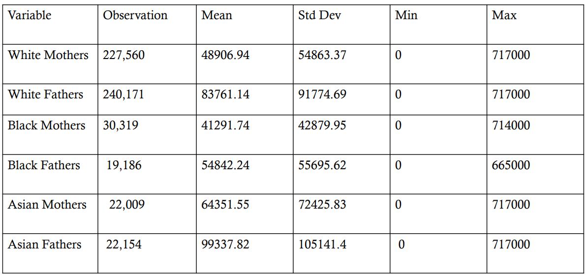
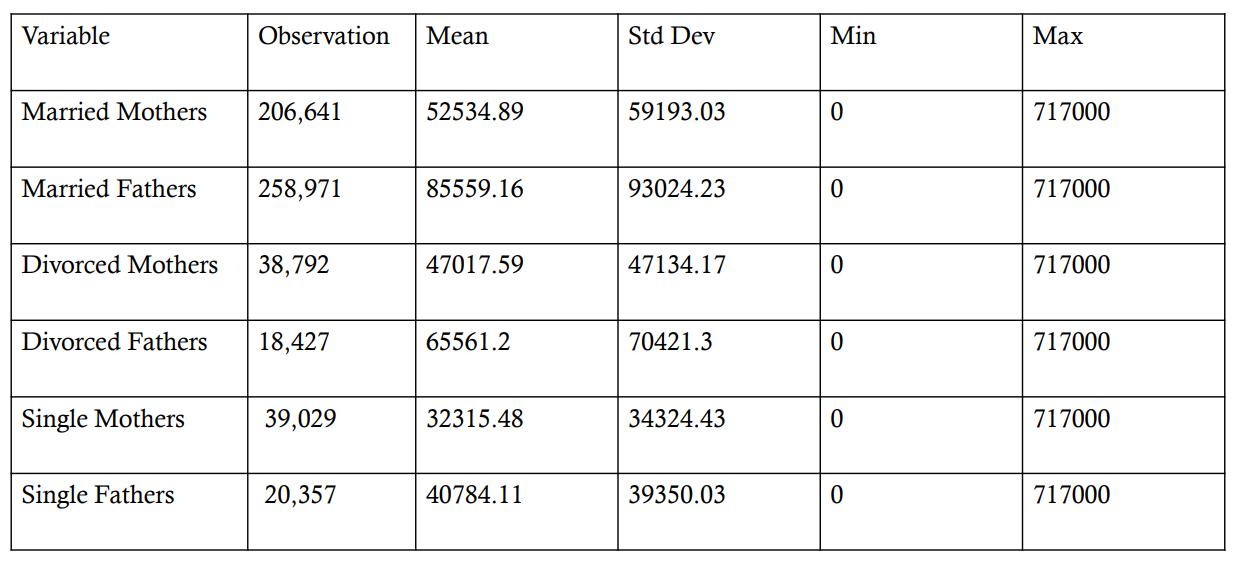 Table 3: Summary Statistics Measuring the Effect of Race on Income
80
Table 4: Summary Statistics Measuring the Effect of Marital Status on Income
Table 5: Summary Statistics Measuring the Effect of Education on Income
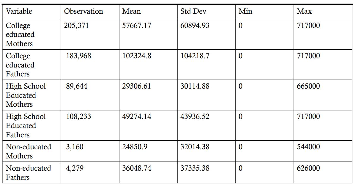
5.0 CONCLUSION
In summary, the estimates obtained by the study demonstrates that the impact of a child on a man is positively related with a significantly higher income comparatively to that on a woman, which can help explain a proportion of the gender wage gap. The results in this paper imply that race, education, and marital status contribute significantly to the income discrepancies between mothers and fathers. Policy implications, such as paid leave, high quality childcare, and flexible schedules are a vital component in decreasing the motherhood penalty. To create a smaller and potentially non-existent gap the United States should attempt offering paid leave that only fathers are eligible to take. In addition, it is of equal importance to recognize that with the extremely high costs of childcare, it would be beneficial to increase the availability and reduce the of outof-pocket cost for public early care and education. Economically, this can increase labor force participation rate, especially mothers which in turn can reduce the gap. Lastly, this study
81
contributes to extant literature by empirically analyzing the fatherhood bonus as it relates to the motherhood penalty.
82
Appendix A: Variable Description and Data Source
Acronym Description
Incwage Reports each respondent's total pre-tax wage and salary income - that is, money received as an employee - for the previous year.
nchild Counts the number of own children (of any age or marital status) residing with each individual. NCHILD includes stepchildren and adopted children as well as biological children.
age Reports the person's age in years as of the last birthday.
race The race of the individual.
marst Each person's current marital status.
educ Indicates respondents' educational attainment, as measured by the highest year of school or degree completed.
state Identifies the state in which the housing unit was located, using the coding scheme developed by the Inter-University Consortium for Political and Social Research (ICPSR).
Data source
Integrated Public Use Microdata Series (IPUMS)
Integrated Public Use Microdata Series (IPUMS)
Integrated Public Use Microdata Series (IPUMS)
Integrated Public Use Microdata Series (IPUMS)
Integrated Public Use Microdata Series (IPUMS)
Integrated Public Use Microdata Series (IPUMS)
Integrated Public Use Microdata Series (IPUMS)
83
BIBLIOGRAPHY
Anderson, D. J., Binder, M., & Krause, K. (2002). The motherhood wage penalty: Which mothers pay it and why?. American economic review, 92(2), 354-358.
Benard, S., & Correll, S. J. (2010). Normative discrimination and the motherhood penalty. Gender & Society, 24(5), 616-646.
Combet, B., & Oesch, D. (2019). The gender wage gap opens long before motherhood. Panel evidence on early careers in Switzerland. European sociological review, 35(3), 332-345.
Cowan, J., & Kamarck, E. C. The Fatherhood Bonus and The Motherhood Penalty: Parenthood and the Gender Gap in Pay.
Hodges, M. J., & Budig, M. J. (2010). Who gets the daddy bonus? Organizational hegemonic masculinity and the impact of fatherhood on earnings. Gender & Society, 24(6), 717-745.
Jee, E., Misra, J., & Murray‐Close, M. (2019). Motherhood Penalties in the US, 1986–2014. Journal of Marriage and Family, 81(2), 434-449.
Kahn, J. R., García-Manglano, J., & Bianchi, S. M. (2014). The Motherhood Penalty at Midlife: Long-Term Effects of Children on Women's Careers. Journal of marriage and the family, 76(1), 56–72. https://doi.org/10.1111/jomf.12086
Kliff, S. (2018, February 19). The True Cause of the Gender Wage Gap. Vox. Retrieved May 1, 2022, from https://www.vox.com/2018/2/19/17018380/gender-wage-gap-childcare-penalty
Looze, J., & Desai, S. (2020). Economic Engagement of Mothers: Entrepreneurship, Employment, and the Motherhood Wage Penalty. Employment, and the Motherhood Wage Penalty (December 19, 2020).
Lundberg, I. (2012). Gender-differentiated effects of parenthood on earnings: understanding Cross-National Variation in the Motherhood Penalty and Fatherhood Bonus (No. 576). LIS Working Paper Series.
Nizalova, O. Motherhood wage penalty may affect pronatalist policies. IZA World of Labor 2017: 359 doi: 10.15185/izawol.359
84
The Empirical Analysis of Motherhood Penalty: The Effect of Having Children on Women’s Career
Madison Henrya
Abstract:
This paper investigates the motherhood penalty as well as the fatherhood bonus. The Motherhood penalty is a phenomenon by which women’s pay decreases once they become mothers. The fatherhood bonus refers to the advantages that working fathers get in terms of pay and perceived competence in comparison with working mothers and childless men This study incorporates information on the effect a child has on a mother’s income verse that of a father’s, while also measuring how a woman’s income is affected after having a child comparatively to that of a childless woman’s. The results show that the income of Mother’s was higher than that of non-mothers, but more glaringly, results showed fathers making substantially more than mothers which could more accurately explain the gender wage gap.
JEL Classification: J13, J16
Keywords: Motherhood Penalty, Fatherhood Bonus.
a Student, Bryant University, 1150 Douglas Pike, Smithfield, RI02917. Phone: (484) 832-0658.
Email: mhenry4@bryant.edu.
85
1.0 INTRODUCTION
Despite mothers’ high rates of labor force participation and the reliance of households on mothers’ paid and unpaid work, many mothers do not have the support they need. This causes mothers to face considerable difficulty balancing caregiving and family responsibilities with economic participation. Though childbearing has economic benefits for our society, women are financially penalized for having children, which commonly referred to as the motherhood penalty.
This study aims to enhance understanding on how women’s careers are impacted by having a child From a policy perspective, this analysis is important because it validates the necessity for paid parental leave since, the United States, unlike most developed countries worldwide, does not guarantee paid annual leave, paid parental leave, or paid time off for illness or family care. The relevance of this study is that woman comprise almost half of the U.S. labor force, and many of those women are mothers, mothers whom earning potential is negatively affected just for having children. If ignored, it may undermine policy initiatives aiming to increase fertility rates in post-socialist countries, such as the costly “baby bonus,” which is a government payment to new parents to assist with the costs of childrearing Nizalova (2017).
A child can greatly shift the economics of a household. Mothers’ unpaid work is also crucial to their households and the economy. Mothers spend more time than fathers
“orchestrating family life,” including caring for children, transporting them to school and other activities, and doing housework. Despite the importance of mothers’ economic contributions, the broader economy fails to support mothers in a variety of ways. The well-being of children is not only important for families, but also the future of the economy. Policies such as paid leave, affordable and high-quality childcare, and flexible schedules enable mothers to remain connected
86
to the labor market both as employees and as entrepreneurs gives motherhood the economic support that it needs.
This paper was guided by three research objectives: How is a woman’s income effected by children? How is a woman’s vs a male’s income effected by the addition of a child? How does the race/ethnicity, education level, and marital of a woman vs a male effect the motherhood penalty/fatherhood bonus comparatively?
The rest of the paper is organized as follows: Section 2 gives a brief literature review. Section 3 outlines the empirical model. Data and estimation methodology are discussed in section 4. Finally, section 5 presents and discusses the empirical results. This is followed by a conclusion in section 6.
2.0 TRENDS
Figure 1 shows that women with kids suffer a decrease in earning after the birth of their first child while males’ earnings stay rather constant. Henrik Kleven, an economist at Princeton University who conducted this study, suggests what we often think of as a gender pay gap is more accurately discussed as a childbearing pay gap or motherhood penalty, which is illustrated in Figure 2. Childless women have earnings that are quite similar to men’s salaries, while mothers experience a significant wage gap
87
Figure 1: Effect of a Child on Women vs Men
Source: Children and Gender Inequality: Evidence from Denmark; National Bureau of Economic Research
Figure 2 shows the different earning trajectories for women who have children versus those who do not become mothers. The study estimated that childbearing, accounts for 80 percent of the gender wage gap in Denmark. Similar studies conducted in the United States have found similar results. For example, Harvard economist Claudia Goldin has found that women in their 30s incur the largest gender wage gap in America, which is their prime, childbearing years.
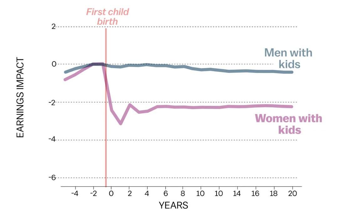
88
Source: Children and Gender Inequality: Evidence from Denmark; National Bureau of Economic Research
Figure 3 shows first the wage penalty for one child, the gross penalty was 16.9% in 1986 to 1995 and 17.3% in 2006 to 2014. The penalty net of differences in education was 9.5% in 1986 to 1995 and 14.5% in 2006 to 2014, and the penalty net of differences in education and labor market experience was 8.2% in 1986 to 1995 and 13.7% in 2006 to 2014. Figure 1, suggest an economically significant decrease in the pay of mothers of one child relative to childless women with comparable human capital. The gross penalty for two children was 24.5% in 1986 to 1995 and 18.8% in 2006 to 2014. The penalty net of education was 17.8% in 1986 to 1995 and 15% in 2006 to 2014. As mothers of two children improved their education and labor market experience, over time, the gross gap between their wages and the wages of childless women appears to have decreased. The net gap, the gap due to factors other than human capital, however possibly including labor market discrimination against mothers or unobservable differences in labor market productivity between mothers and childless women remained stable. The results for
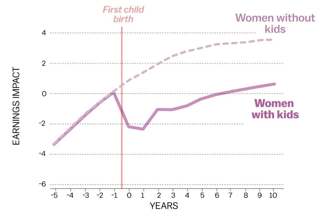
Figure 2: Motherhood Penalty
89
mothers of three or more children were similar to those for mothers of two children. The gross penalty for three or more children declined from 35.9% in 1986 to 1995 to 31.1% in 2006 to 2014, although this change was not statistically significant. When comparing women with the same level of education and experience, mothers with three or more children saw a stable wage penalty over time.
Source: Motherhood Penalties in the U.S., 1986–2014
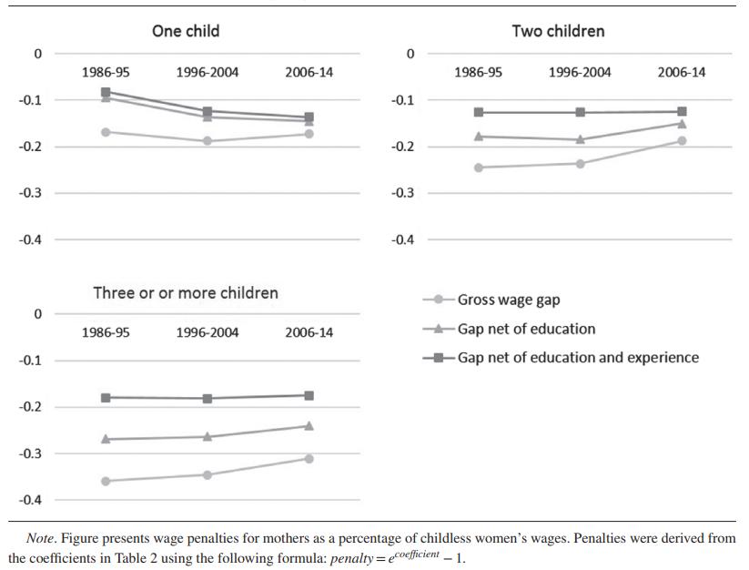 Figure 3: Wage Penalties for One, Two, and Three or More Children Compared with No Children
90
Figure 4 shows that only nine states, New York, New Jersey, Rhode Island, Washington D.C, Washington, California, Colorado, Connecticut, Massachusetts and Oregon enacted family and medical paid leave laws. This is important because studies show that paid family leave helps keep women linked to the labor market, which in turn can negate motherhood wage penalty because women would not be completely removed from paid work. The introduction of paid family leave in California and New Jersey was found to increase mothers’ labor force attachment in the year of birth and up to five years afterward. For mothers with college degrees, the effects lasted closer to eight years. Moreover, paid maternity leave is also associated with higher pay among mothers. Wages of mothers who were working prior to the birth of their first child and received pay during their maternity leave are 9% higher than those of other mothers.
Source: Economic Engagement of Mothers: Entrepreneurship, Employment, and The Motherhood Wage Penalty
 Figure 4: States who Have Paid Family Leave
91
3.0 LITERATURE REVIEW
The motherhood penalty is used to describe the economic effect on a woman when she has a child. According to Jee et al. (2019) previous studies found that mother earn less than childless women. Two studies found that employed mothers in the United States suffer a per-child wage penalty of approximately 5%, on average, after controlling for the usual human capital and occupational factors that affect wages Budig and England 2001; Anderson et al. (2003). Kahn et al. (2015) provides argument for this effect stating that having and raising children interferes with the accumulation of human capital, which translates to levels of productivity and in turn lower wages. Research indicates that Women who, as a result of having or planning to have children, either cut short their education, drop out of the labor force for an extended period, cut back to part-time employment, choose occupations that are more family friendly, devote less effort on the job, or pass up promotions because of time or locational constraints, end up achieving less than childless women who stay on track with full-time employment and take advantage of opportunities for training and career advancement. Prior research, such as Budig and England (2001), showed a 7% per-child penalty using data from the National Longitudinal Survey of Youth (NLSY). They argued that only one third of this penalty can be attributed to lost experience yet using data from the PSID, Lundberg and Rose (2000) suggested that experience plays a key role, arguing that mothers only face penalties when they interrupt their employment due to care responsibilities. In terms of productivity, William (2001) found that mothers were offered salaries 7.9% less than childless women, whereas actual prospective employers called mothers back for interviews half as often as they did childless women, which was research based on both a laboratory experiment and a real-world audit study with actual employers Correll et al.
92
(2007). This research suggests that employers’ perceptions of mothers as less committed to work may help account for the motherhood penalty, even when there do not appear to be warranted reasons to discriminate against mothers Jee et al. (2019).
Therefore, another explanation for the Motherhood penalty is mothers may face workplace discrimination because some employers believe that mothers are less competent or committed to their jobs than childless women, however this discrimination is hard to measure Kahn et all. (2015). Using residual wage differences that remain after controlling for human capital and other relevant characteristics Correll et al. (2007) is an alternate and effective way to capture such discrimination.
Studies also showed the evaluation of the motherhood penalty through education level. For example, Anderson et al. (2003) compared the motherhood wage penalty for mothers in different educational groups and found that mothers who were high school graduates experienced the largest wage penalty. They interpret the relationship between level of education and the magnitude of the wage penalty as evidence contradicting productivity explanations of the motherhood wage penalty. However, the authors lack direct measures of productivity, limiting their ability to rule out productivity explanations Correll et al. (2007). Moreover, Anderson et al. (2002) research found that the motherhood wage penalty for white mothers varies considerably by education level. In a cross section, mothers who did not complete high school do not earn less than their childless counterparts, while high-school and college graduates earn about 10 percent less per child. Anderson et al. (2002) research concluded that the least skilled do not suffer lower wages for becoming mothers, there is a 15-percent penalty for college-educated mothers of two
93
or more children, which can be entirely explained by years out of the workforce for whites, and that women who are high school graduates and black college graduates appear to occupy a middle position: years out of the workforce contribute only modestly to explaining the motherhood wage penalty experienced by individual women.
4.0 DATA AND EMPIRICAL METHODOLOGY
4.1 Data
The study uses annual panel data from 2019. Data was obtained from the Integrated Public Use Microdata Series (IPUMS). Publicly available. Summary statistics for the data are provided in Table 1.
Table 1 Summary Statistics
4.2 Empirical Model
Variable Observation Mean Std. Dev. Min Max Incwage 1,402,150 56104.47 68118.78 0 717000 nchild 1,402,150 .8019049 1.114506 0 9 age 1,402,150 42.1215 13.33417 16 65 white 1,402,150 779172 4148049 0 1 black 1,402,150 0837692 .2770415 0 1 asian 1,402,150 0643982 2454611 0 1 mwspouse 1,402,150 544961 4979746 0 1 separated 1,402,150 0163385 .1267736 0 1 divorced 1,402,150 .104665 .3061214 0 1 widowed 1,402,150 .0134572 .115222 0 1 single 1,402,150 .0162282 .2303629 0 1 noschooling 1,402,150 .0150526 .1217622 0 1 highschool 1,402,150 .3550162 .4785184 0 1 college 1,402,150 .6205035 .4852619 0 1 94
Following Anderson, Binder Krouse (2009) this study adapted and modified Motherhood Penalties in the U.S., 1964-2014 Jee et al. (2019). The model could be written as follow:
Incwage is the annual amount of total income for the individual It represents total pre-tax wage and salary income, that is, money received as an employee, for the previous year.
Independent variables consist of five variables obtained all from IPUMS. Appendix A provide data source and descriptions, for using the variables. First, nchild is a dummy variable and represents the presence of a child in the household. Second, Age is the age of the induvial.
All the research done in this study used individuals 65 or under. Third, race is a dummy variable and was categorized into White, Black, and Asian. Fourth, marst is a dummy variable signifying the individual’s marital status and categorized into married, separated, divorced, single, and widowed. Fifth, educ is a dummy variable measured by the highest year of school or degree completed and categorized into college, high school, or no education. Lastly, state identifies the state in which the housing unit was located of the individual.
5.0 EMPIRICAL RESULTS
The empirical estimation results are presented in Table 2. The empirical estimation showed that nchild had a relatively strong and significantly positive effect at the 1% level on Incwage for both women and men. Fixed effect with state shows parallel results; had a relatively strong and

95
significantly positive effect at the 1% level on Incwage for both women and men. Results were only gathered on individuals under the age of 65 and who were currently employed. Interpreting these results, it is evident that women with children make more then women without children and men with children make more then men without children. This does not align with current literature, however because of limitations in the study including only accounting for the year 2019 and not measuring the impact of income before and after a child, could be reason why. Most glaringly in the results was the fatherhood bonus, men with children made over four thousand more than women with children. This is consistent with the results of Hodges and Budwig (2010) who further suggested the gender wage gap should be more accurately discussed as the motherhood penalty. For further analysis, Tables 3, 4 and 5 looks at the effects of race, education, and marital status on a mother’s income comparatively to that of fathers. Table 3 results, finding that white fathers earn roughly $34,854 thousand more than white mothers; Black fathers earn roughly $13,550 thousand more than Black mothers and Asian fathers earn roughly $34,986 more than Asian mothers, is consistent with Loose and Desai (2020) study that concluded the motherhood wage penalty is larger among white women, and children have smaller effects on the wages of Black women. Moreover, results measuring the effects of marital status on a mothers’ income verse that of fathers, as seen in Table 4, show that married fathers earn roughly $33,025 more then married mothers; divorced fathers earn roughly $18,544 more then divorced mothers; and single fathers earn roughly $8,469 more than single mothers. Lastly, Table 5 measures the effect of education on the income of mothers compared to that of fathers and show that fathers with a college degree or higher earn $44,657 more then mothers with a college degree or higher; Fathers who highest educational attainment was a high school diploma
96
earn roughly $19,969 more then mothers with the same status; Fathers without any education making $11,198 more than mothers without an education.
97
Table 2: Regression results for the Motherhood Penalty and Fatherhood Bonus
Note: *** , **, and * denotes significance at the 1%, 5%, and 10% respectively. Standard errors in parentheses
Dependent Variable = Income I Women with Children II Women with Children III Men with Children IV Men with Children CONSTANT -9352.545*** (733.0255) -915.817 (913.5573) -28512.01 (909.4048) -13000.91 (91214.837) age 550.7929*** (5.464708) 524.2984*** (5.433801) 834.5962 *** (7.896936) 810.0572*** (7.864337) nchild 468.089 *** (59.31744) 391.2826*** (58.88842) 4362.622*** (85.04443) 4276.861*** (84.61492) mwspouse 6788.22 *** (172.6349) 8097.097*** (171.9128) 21517.19*** (254.1749) 22649.19*** (253.3576) college 32503.29*** (682.3376) 32638.73*** (676.8575) 51295.91*** (833.6765) 51589.43*** (828.6697) white 3135.659*** (238.6553) 5630.667*** (241.6314) 9509.974*** (334.4778) 12707.33*** (339.3611) black 139.946 (299.4371) 2170.236*** (305.749) -6315.142*** (450.6245) -4584.831*** (457.8487) asian 14997.92*** (326.4184) 13216.77*** (325.6813) 17559.33*** (471.1528) 15565.91*** (470.2301) gradeschool -2696.092*** (884.9168) -3216.676*** (877.6781) -2955.895*** (1034.179) -3073.222*** (1027.515) highschool 7126.245*** (686.5422) 8264.477*** (681.106) 13386.35*** (837.1667) 15168.97*** (832.3346) seperated -1532.495*** (448.6541) -764.6447 (445.2603) 6109.099*** (777.4857) 6630.813*** (772.7505) divorced 3363.983*** (229.9568) 4866.048*** (228.7199) 5239.785*** (363.8649) 7005.373*** (362.3072) mwospouse 2338.254*** (459.325) 2586.568*** (455.6392) 10401.2*** (652.3191) 10323.82*** (648.2036) widowed -4396.738*** (452.7115) -2705.147*** (449.3731) 1128.585 (1070.829) 2894.594*** (1064.187) R2 0.0970 0.1121 0.1443 0.1556 F-statistics 5580.01*** 1353.27*** 9426.21*** 2125.05*** Number of obs. 675,414 675,414 726,736 726,736 Fixed effect with State NO YES NO YES
98
Table 3: Summary Statistics Measuring the Effect of Race on Income
99
Table 4: Summary Statistics Measuring the Effect of Marital Status on Income
Table 5: Summary Statistics Measuring the Effect of Education on Income
5.0 CONCLUSION
In summary, the estimates obtained by the study demonstrates that the impact of a child on a man is positively related with a significantly higher income comparatively to that on a woman, which can help explain a proportion of the gender wage gap. The results in this paper imply that race, education, and marital status contribute significantly to the income discrepancies between mothers and fathers. Policy implications, such as paid leave, high quality childcare, and flexible schedules are a vital component in decreasing the motherhood penalty. To create a smaller and potentially non-existent gap the United States should attempt offering paid leave that only fathers are eligible to take. In addition, it is of equal importance to recognize that with the extremely high costs of childcare, it would be beneficial to increase the availability and reduce the of outof-pocket cost for public early care and education. Economically, this can increase labor force participation rate, especially mothers which in turn can reduce the gap. Lastly, this study
100
contributes to extant literature by empirically analyzing the fatherhood bonus as it relates to the motherhood penalty.
101
Appendix A: Variable Description and Data Source
Acronym Description
Incwage Reports each respondent's total pre-tax wage and salary income - that is, money received as an employee - for the previous year.
nchild Counts the number of own children (of any age or marital status) residing with each individual. NCHILD includes stepchildren and adopted children as well as biological children.
age Reports the person's age in years as of the last birthday.
race The race of the individual.
marst Each person's current marital status.
educ Indicates respondents' educational attainment, as measured by the highest year of school or degree completed.
state Identifies the state in which the housing unit was located, using the coding scheme developed by the Inter-University Consortium for Political and Social Research (ICPSR).
Data source
Integrated Public Use Microdata Series (IPUMS)
Integrated Public Use Microdata Series (IPUMS)
Integrated Public Use Microdata Series (IPUMS)
Integrated Public Use Microdata Series (IPUMS)
Integrated Public Use Microdata Series (IPUMS)
Integrated Public Use Microdata Series (IPUMS)
Integrated Public Use Microdata Series (IPUMS)
102
BIBLIOGRAPHY
Anderson, D. J., Binder, M., & Krause, K. (2002). The motherhood wage penalty: Which mothers pay it and why?. American economic review, 92(2), 354-358.
Benard, S., & Correll, S. J. (2010). Normative discrimination and the motherhood penalty. Gender & Society, 24(5), 616-646.
Combet, B., & Oesch, D. (2019). The gender wage gap opens long before motherhood. Panel evidence on early careers in Switzerland. European sociological review, 35(3), 332-345.
Cowan, J., & Kamarck, E. C. The Fatherhood Bonus and The Motherhood Penalty: Parenthood and the Gender Gap in Pay.
Hodges, M. J., & Budig, M. J. (2010). Who gets the daddy bonus? Organizational hegemonic masculinity and the impact of fatherhood on earnings. Gender & Society, 24(6), 717-745.
Jee, E., Misra, J., & Murray‐Close, M. (2019). Motherhood Penalties in the US, 1986–2014. Journal of Marriage and Family, 81(2), 434-449.
Kahn, J. R., García-Manglano, J., & Bianchi, S. M. (2014). The Motherhood Penalty at Midlife: Long-Term Effects of Children on Women's Careers. Journal of marriage and the family, 76(1), 56–72. https://doi.org/10.1111/jomf.12086
Kliff, S. (2018, February 19). The True Cause of the Gender Wage Gap. Vox. Retrieved May 1, 2022, from https://www.vox.com/2018/2/19/17018380/gender-wage-gap-childcare-penalty
Looze, J., & Desai, S. (2020). Economic Engagement of Mothers: Entrepreneurship, Employment, and the Motherhood Wage Penalty. Employment, and the Motherhood Wage Penalty (December 19, 2020).
Lundberg, I. (2012). Gender-differentiated effects of parenthood on earnings: understanding Cross-National Variation in the Motherhood Penalty and Fatherhood Bonus (No. 576). LIS Working Paper Series.
Nizalova, O. Motherhood wage penalty may affect pronatalist policies. IZA World of Labor 2017: 359 doi: 10.15185/izawol.359
103
A Panel Data Analysis of Institutional Quality, FDI, and Public Debts’ Impact on Economic Growth for ASEAN
Joshua Kearneya
Abstract:
This paper investigates the effects on economic growth driven by institutional quality, foreign direct investment, and public debt while doing a breakdown and comparison between the first and last five nations to join ASEAN as well as a collective analysis of the complete 10 ASEAN. The model used in this paper focuses primarily on the country’s gross domestic product and the domestic growth seen within ASEAN that utilized public debt to fund governmental agendas.
JEL Classification: F16, O4, P45
Keywords: Public debt, Economic Growth, Institutional Quality, ASEAN, Foreign Direct Investment
a Student, Bryant University, 1150 Douglas Pike, Smithfield, RI02917. Phone: (860) 951-9717. Email: jkearney2@bryant.edu.
104
Economic growth has played a key role in the advancement of the Association of Southeast Asian Nations (ASEAN). From a conventional perspective, countries that increase their public debt to finance their government's deficit can stimulate aggregate demand and economic performance in the short term. In a situation where there is not strict control over the amount of debt that is accumulated, the experience in the long term could result in capital outflows and a level of reduction in a country's important output (Herrera et al. 2017).
This study aims to enhance the understanding of the implication that ASEAN faces when utilizing public debt to finance their economic and governmental operations and programs. From a policy perspective, this analysis is important because the relationship between a country's institutional quality and its economic growth can significantly be impacted or altered due to a country's level of outstanding public debt. The relevance of this study is that it allows for investors and economists to understand the fundamental strengths of a nation and analyze countries' need for debt-financed expansionary fiscal policy in times of slow growth or to maintain strong and stable economic growth in the short and long-term future.
Economists have long debated the effects of economic growth that can be achieved through utilizing public debt. Some studies have suggested that in times of crisis expansionary fiscal policy should be implemented to maintain or continue a country's growth trajectory, while others indicate that increasing levels of public debt will significantly reduce economic performance and therefore should be avoided (Herrera et al. 2017).
This research was guided by three research objectives. First, it investigates how public debt, institutional quality, and foreign direct investment will affect economic growth for the ASEAN 10. Second, this research will investigate how ASEAN 5 has been able to see growth and economic improvements within their countries. Lastly, the research will investigate how ASEAN 10 compares to the growth of the ASEAN 5 as the shift of demand, labor, and foreign direct investment are changing.
1.0
INTRODUCTION
105
2.0 TREND (OF THE GIVEN TOPIC)
Figure 1 shows a preliminary summary of potential economic growth from the sample of new and old member states within the European Union. The graph shows the average GDP growth rate across different public debt levels in different EU member countries.
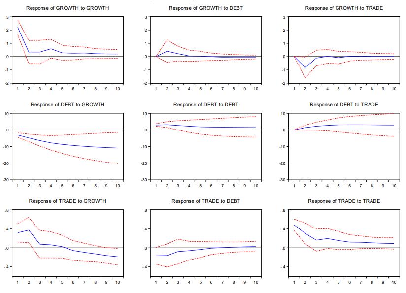
Source: WDI, 2012; OECD, 2013. Calculations: (Mencinger et al., 2014)
Figure 2 shows the results of when public debt rises in Japan. When public debt rises, the economic growth rate for Japan is hurt and can be seriously damaged. You will also see that in Figure 2 that a country's openness helps expand the economy, but this expansion is short-lived.
Source: (Kurihara, 2015)
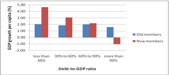 Figure 1: Relationship Between GDP growth per capita and different levels of public debt for old and new EU member states
Figure 2: Impulse Response Function
Figure 1: Relationship Between GDP growth per capita and different levels of public debt for old and new EU member states
Figure 2: Impulse Response Function
106
Currently, ASEAN 5 has been seeing the trend of high-tech exports in comparison to the newest five members in ASEAN. This trend can be seen in figure 3. Figure 3 shows ASEAN 5 and the level of high-tech exports as a percentage of manufactured exports for each of the five nations.
High-technology exports (% of manufactured exports) ASEAN 5
3.0 LITERATURE REVIEW
Foreign direct investment (FDI) is believed to be the most crucial to economic growth and enhancement. Higher levels of FDI typically can be a driver for a larger amount of technological advancement as well as exposure to existing knowledge and transfer of knowledge (Almeria et al. 2014). By employing the system Generalized Method of Moments (SGMM) used in (Nguyen et al. 2018), there is a significantly positive impact of institutional quality on a country's economic growth. It is likely the institutional quality can be derived from higher levels of FDI as well as trade openness by the country. The importance of this economic growth is not only to represent the growth of a country but also is essential to maintain and improve the international
Figure 3: High Technology Exports as a Percentage of Exports for ASAN 5 from 2009 – 2019
Source: The World Bank
8 18 28 38 48 58 68 2009 2010 2011 2012 2013 2014 2015 2016 2017 2018 2019 Percent of Manufacted Exports Year
Indonesia Malaysia Philippines Singapore Singapore Thailand 107
competitiveness a country has in a global environment. The drivers of institutional quality that will proceed to further develop and strengthen a country's economic growth can be found through various variables that display a country's level of political stability, regulatory quality, government effectiveness, perceived corruption, and numerous other indicators that display country stability and strength (Kandil 2009).
While this paper and research investigate the economic growth of all 10 ASEAN countries, the first five countries to join this alliance are more developed than the later five that have joined. The research found by (Herrera et al. 2017) work develops an understanding of how different income groups have different levels of economic growth. The results of this research showed that countries that have the lowest levels of public debt are characterized by having the highest levels of economic growth while the countries with the higher levels of public debt showed the smallest levels of economic growth. After analyzing countries by income level, the research suggested that there is not a clear pattern between public debt and economic growth, but it indicated that there was a heterogeneous relationship. Using the International Monetary Fund’s classification of low-income countries, lower-middle-income countries, upper-middle-income countries, and high-income countries the results do not suggest a clear pattern in public debt and economic growth across different countries. While conducting research there is an argument that different time frames yield different results. The long-term results (Emmanuel 2012) show that the joint impact of debt on economic growth is negative and is deemed significant while the short-term impact of public debt and borrowing funds and the coefficient of a budget deficit are positive.
Again, looking back at the research between developed and undeveloped countries there is an indication that there is a negative relationship between the public debt and economic growth. In the study done on Japan, the researchers found that the trade openness of a country's economy is not necessarily related to strengthening a country's economic growth. This study also found that debt should be avoided and, in the future, should be reduced, which is vital and necessary to continue strong economic growth for Japan's economy (Kurihara 2015). The impacts of short-term country debt
108
have been further researched with the developments when doing an analysis on countries in the European Union (EU) showing that there is a significant non-linear impact of public debt on debt ratios and GDP per capita growth rates. This research and study also suggest that the old member states within the EU have a higher threshold before public debt inverts into a negative effect while newer member states have a lower turning point (Mencinger et al. 2014).
4.0 DATA AND EMPIRICAL METHODOLOGY
4.1 Data
The study uses annual panel data set from 2009 to 2019. Data was obtained from The World Bank website and the World Development Index website. When acquiring the data, this study utilized proxies to develop a model that would take into account institutional quality by accessing The World Bank’s Worldwide Governance Indicators. The two proxies utilized were Voice/accountability which measures the extent to which citizens can select their government as well as freedom of expression, media, and association. The second proxy is used for government effectiveness. Government effectiveness measures the quality of the goods and services provided by the government as well as the degree of independence the government has from political pressures. Both variables combined to allow for the model to incorporate institutional quality in the regression results.
Table 1 Summary Statistics
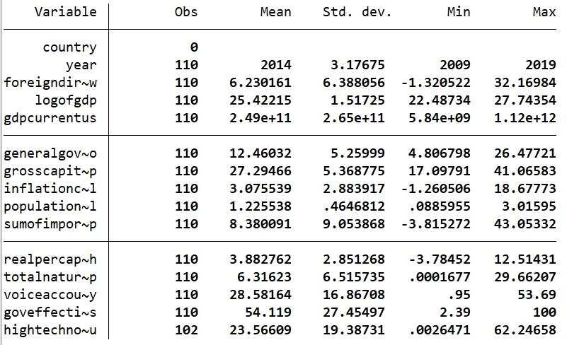
109
4.2 Empirical Model
Following (Lartey et al. 2018) this model has been adapted and modified by dropping the quadratic term for government debt and adding four independent variables, natural resource rent, Voice/accountability, government effectiveness, high-tech exports.
The model could be written as followed:
GDPG is the real gross domestic product growth rate i at year t. GDPG is used to measure the amount of economic growth that is represented within the ASEAN countries. The real GDP growth rate is the final market value of goods and services within a given year when valued at a constant price (Burda and Wyplosz 2009). The beginning of calculating regular estimates of GDP started in the early 1940s (Dynan and Sheiner 2018). While finding the calculation of a country's gross domestic product there are five separate variables you need to find the sum of. First, you need to find a country's private consumption followed by their gross private investment, government investment, government spending, and lastly their exports minus their imports.
GOVD is a country's gross domestic debt that is measured as a percent of its gross domestic product. GROVE is government consumption expenditure as a percent of the country’s gross domestic product. This variable will show the quantity the government consumes in comparison to their GDP. This variable is explained as a governmental fixedterm legally binding commitment to others (Lartey et al. 2018) CAPF is gross capital formation as a percentage of GDP. INFL is a country's inflation rate. POPG is population growth measured in percentage i at year t. OPEN is the sum of all net imports and exports for that country measured as a percentage of GDP. This variable is used as a proxy to
(1) GDP = β0 + β1 GOVD + β2 GOVE + β3 CAPF + β4 INFL + β5 POPG + β6 OPEN + β7 FDI + β8 RENTS + β9 VOICE + β10 GOVEFFECT + β11 TECHEXPORT + Ꜫ
110
measure openness to trade. FDI is foreign direct investment for a country as a percentage of GDP. RENTS this measures the total natural resource rents as a percent of gross domestic product. This is used as a proxy to show the wealth of a nation and its reliance on natural resources to drive its economic expansion (Epo and Faha 2020). VOICE measures voice and accountability as a governance indicator. This indicator is used as a proxy to enable this model to measure institutional quality and to help see the effect this has on building strong economic growth. This variable helps explain how some nations in ASEAN have stronger institutional quality than others and shows the direct impact that has on a nation’s economic growth (Kandil 2009). GOVEFFECT is the government effectiveness which reflects a government's ability to have quality public service, civil service, and the degree of its independence from political pressures. This independent variable is used as a proxy for institutional quality (Kandil 2009). Lastly, TECHEXPORT measures a country's high-technology exports as a percent of manufactured exports. This measures the exports of goods that require intensive levels of research and development such as aerospace, computers, and pharmaceuticals. This variable was added to the original model as it captures the difference in development levels between ASEAN 5 and the newest members.
5.0 EMPIRICAL RESULTS
The empirical estimation results are presented in Table 2 and Table 3. This study used OLS, Fixed-effects, and Random-effects regressions to analyze the data. After using the Hausman test, the results showed that the Fixed-effects regression corresponded the best with the data. In Table 2 there are six independent variables that are considered significant at the one percent level. Within Table 3 you will find that there is only one variable that is statistically significant at the one percent level. Overall, the results correspond with previous results found in (Mencinger et al. 2014).
One interesting aspect of this study that can be found to align with previous literature is the different effect that government consumption expenditure has a negative coefficient as related to gross domestic product. This result is consistent with what has been found in the (Kurihara 2015) literature which focuses primarily on Japan. You will also see that when comparing the government consumption expenditure in Table 2 and
111
Table 3, the negative effect is greater on ASEAN-5 rather than ASEAN-10. This is due to the fact that ASEAN-5 nations are considered to be more developed than the newer members. According to the study on Japan by (Kurihara 2015), less developed nations often see greater growth when federal governments spend capital within the nation. In Table 2 you will find that there are six variables that are significant at the one percent level under the fixed effect column. You will also see that under the ordinary least squares model there are eight out of the ten variables considered significant at the one percent level. After running the Hausman test and comparing the different estimators, the results indicated that the fixed effect regression produced the most accurate representation of the data. In Table 3 you will find that there was only one variable in the fixed effect regression that was deemed to be significant at the one percent level, which was high-tech exports. On the other hand, the ordinary least squares regression for ASEAN-5 showed that there are a total of four variables that were significant to gross domestic product growth at the one percent level.
GDP GROWTH OLS FIXED RANDOM CONSTANT .30810*** (.30810) 24.981*** (.36880) 24.278*** (.35999) FDI -.04845*** (.01062) .00820 (.01069) -.08772*** (.00975) GOV’T Consumption Expenditure -.04752*** (.01339) -.05748*** (.01436) -.08814*** (.01351) Gross Capital Formation .00797 (.01019) .01763*** (.00591) .03751*** (.01044) Inflation .07788*** (.01750) .02882*** (.01007) .06745*** (.02045) Population Growth -.93131*** (.11473) -.18368*** (.08028) -1.2015*** (.12362) Sum of Imports and Exports .01189** (.00549) -.01530*** (.00359) .01661*** (.00638) Natural Resource Rents -.06246*** (.01160) -.01298 (.01063) -.09418*** (.01209) Voice / Accountability .01594*** (.00516) -.00704 (.00496) .03577*** (.00462) 112
Table 2: Regression results for the ASEAN-10
Note: ***, **, and * denotes significance at the 1%, 5%, and 10% respectively. Standard errors in parentheses
Results that I found to be most interesting from my analysis of these regressions are from Table 2 and Table 3. In Table 2 and Table 3 the coefficient of government
Government Effectiveness .01413*** (.00379) .00983* (.00511) .02190*** (.00441) High-Tech Exports .01866*** (.00393) .02353*** (.00448) .01067*** (.00434) R2 .9432 .5955 .1582 F-statistics 0.0000 0.0000 Number of obs. 102 102 102
Table 3: Regression Results for ASEAN-5
OLS FIXED RANDOM CONSTANT 29.917*** (29.817) 24.199*** (1.144) 28.272*** (.61793) FDI -.01653** (.00689) .01472 (.02163) -.00113 (.02492) GOV’T Consumption Expenditure -.16278*** (.02410) -.07046** (.02616) -.10090*** (.01166) Gross Capital Formation .03054** (.01448) .01725** (.00819) .01561 (.00973) Inflation .00920 (.01830) .03411** (.01448) .02828* (.01453) Population Growth -.33430*** (.06439) -.05904 (.55675) -2.9199*** (.25116) Sum of Imports and Exports -.01291*** (.00391) -.02116** (.00904) -.02709*** (.00873) Natural Resource Rents .01354 (.00934) -.01735 (.01749) -.00331 (.01335) Voice / Accountability -.01730** (.00634) -.00644 (.00932) .00033 (.01055) Government Effectiveness -.00603*** (.00330) .00834 (.00919) .00199 (.00433) High-Tech Exports -.00588** (.00272) .02443*** (.00704) .02519*** (.00531) R2 .9445 .6299 .3519 F-statistics 0.0000 0.0000 Number of obs. 47 55 55 113
GDP GROWTH
consumption expenditure and population growth both carry a negative sign. The negative sign of these coefficients suggests that when both ASEAN 5 and ASEAN 10 increase their government consumption expenditure by one, there is a -.05748 for GDP growth for ASEAN 10 and a -.07046 for ASEAN 5. These results suggest that the negative impact on a government consumption expenditure is greater for ASEAN 5 over the complete ASEAN 10. The regression results show that an increase in population growth by one has a -.18368 for ASEAN 10 and a -.05904 for ASEAN 5. These results suggest that population growth for ASEAN 10 has a more significant negative impact on GDP growth than it does for ASEAN 5. These results are consistent with the findings of (Mencinger et al. 2014).
5.0 CONCLUSION
In summary, this study has expanded on the vast research that has been conducted on the impacts of variables of institutional quality, public debt, and foreign direct investment and the impact they have on ASEAN 5 and ASEAN 10’s economic growth. The results suggest that for these nations to strengthen their economic growth they must use polices that look to increase factors such as foreign direct investment, capital formation, and maintain an ethical and aware government. These results also suggest that inflation, if produced in a sustainable and contained environment can produce positive effects on both ASEAN 5 and ASEAN 10. The policy implications that this research suggests is for federal and local governments to maintain policies that enforces ethical behavior among law makers and federal agencies. Policies should also look to improving a nations institutional quality and look to increase foreign direct investment. This study also suggests that public debt offers diminishing returns for countries when trying to grow their gross domestic product. In the short-term, public debt can be found to show greater growth in countries but it is short-lived (See Figure 2). These results are also found to be consistent with the research done for Japan in (Kurihara 2015).
Overall, the results of this study suggest that the relationship between economic growth and key macroeconomic variables often has a heterogeneous relationship, leaving
114
the results of this topic left from being conclusive. What results have stated is that countries with different income levels do not show a clear pattern between public debt and economic growth.
Appendix A: Variable Description and Data Source
Acronym Description
GDP
Gross domestic product. This is the total value of goods and services produced in a country for one year.
Data source
World Development Indicators
GOVD Gross domestic debt as a percentage of their GDP
The World Bank
World Development Indicators GOVE Government consumption expenditure as a percent of the country’s gross domestic product
CAPF
Gross capital formation as a percentage of GDP
INFL A countries inflation rate
POPG
OPEN
Population growth measured in percentage
The sum of all net imports and exports for that country measured as a percentage of GDP
FDI foreign direct investment for a country as a percentage of GDP
RENTS
Total natural resources rents (% of GDP) used as a metric to measure institutional quality and shows the difference between the cost of producing a natural resource and the price it can sell it for
The World Bank
The World Bank
The World Bank
The World Bank
The World Bank
The World Bank
VOICE
Voice/Accountability that is used as a proxy to measure policy quality
The World Bank
115
GOVEFFECT Government effectiveness is used as a proxy to measure institutional quality
TECHEXPOR T High-technology exports (% of manufactured exports) is used as a proxy to measure institutional quality
The World Bank
The World Bank
Appendix B- Variables and Expected Signs
Acronym Variable Description What it captures Expected sign
GOVD Gross domestic debt as a percentage of their GDP
The amount of domestic debt a country has compared to their gross domestic product
-
GOVE
Government consumption expenditure as a percent of the country’s gross domestic product
CAPF Gross capital formation as a percentage of GDP
INFL A countries inflation rate
POPG Population growth measured in percentage
OPEN
The sum of all net imports and exports for that country measured as a percentage of GDP
FDI foreign direct investment for a
The percent of goods and services that a government is purchasing +
The amount of domestic investment a nation has +
The rise in price levels +/-
The speed at which a nation is growing +/-
How easy it is for a nation to trade, how often a nation imports and exports +
The amount of investment from +
116
country
to measure institutional quality and shows + VOICE Voice/Accountability that is used as a proxy to measure policy quality
as a metric to show institutional quality and how public perspective is seen by government + GOVEFFECT Government effectiveness is used as a proxy to measure institutional quality Used as a proxy of institutional quality and how effective the policies set by governments are + TECHEXPORT High-technology exports (% of manufactured exports) is used as a proxy to measure institutional quality Measures development and institutional quality between nations +/117
as a percentage of GDP foreign entities within a nation RENTS Total natural resources rents (% of GDP). The difference between the cost of producing a natural resource and the price it can sell it for Metric
Used
Bibliography
Almfraji, M. A., Almsafir, M. K., & Yao, L. (2014). Economic Growth and Foreign Direct Investment Inflows: The Case of Qatar. Procedia.
Emmanuel, O. O. (2012). An Empirical Analysis of the Impact of Public Debt on Economic Growth: Evidence from Nigeria 197-2005. Canadian Social Science, 154-161.
Epo, B. N., & Faha, D. R. (2020). Natural Resources, Institutional Quality, and Economic Growth: An African Tale. European Journal of Development Research, 99-128.
Herrera, R., Carmen, M., & Rivero, S. (2017). An Empirical Characterization of the Effects of Public Debt on Economic Growth. Applied Economics, 3495-3508.
Kandil, M. (2009). Determinants of Institutional Quality and Their Impact on Economic Growth in the MENA Region. International Journal of Development Issues.
Kurihara, Y. (2015). Debt and Economic Growth: The Case of Japan. Journal of Economics Library.
Lartey, E., Musah, a., Okyere, B., & Yusif, A. (2018). Public Debt and Economic Growth: Evidence from Africa. International Journal of Economics and Financial, 35-45.
Mencinger, J., Aristovnik, A., & Verbic, M. (2014). The Impact of Growing Public Debt on Economic Growth in the European Union. Amfiteqtru Economic Journal, 403-414.
Nguyen, C. P., Su, T. D., & Nguyen, T. V. (2018). Institutional Quality and Economic Growth: The Case of Emerging Economies. Theoretical Economic Letters, Vol. 8 No. 11.
118
An Empirical Analysis on Disparities in Access to Healthcare in New York City
Olivia Lemire
Abstract: Healthcare access varies across demographics. Access to healthcare is a strong determinant of health of individuals in New York City. There are a wide range of disparities in health care access for People of Color. Determinants of insurance include race, sex, education status, marital status, whether an individual has children. White individuals, specifically White females have the highest rate of insurance, while Latinx males have the lowest rate of insurance.
JEL Classification: L13, L14
Keywords: Healthcare Access, Inequalities, Racial Disparities
119
The American Hospital Association defines essential health services as primary care, psychiatric and substance use treatment services, emergency department and observation use, prenatal care, transportation, diagnostic services, home care, dentistry services. The Heath Care and Social Assistance industry is the largest employer in New York City, as well as the nation. In the past decade, health insurance expansion has been a major aspect of health reform in the United States. This includes the Patient Protection and Affordable Care Act increasing their coverage to more than 20 million adults in the United States. One study found that 91.7% of their participants have a health care provider while 70.1% of individuals with Medicare are satisfied with the care they receive. Overall, individuals covered by employer sponsored private insurance were less satisfied with their care compared with those covered by Medicare. Those individuals who had a form of private insurance were more likely to report medical debt compared to individuals that are covered by public insurance (Wray et al. 2021).
Roughly 12% of New Yorkers are uninsured. Across the United States health and social inequalities persist, resulting in effects on wellbeing and life expectancy. This is particularly true for large urban areas that having growing income inequalities (Romero et al. 2018). In the case of Brooklyn, New York, many factors influencing health include physical and socio economic, as well as access to clinical care. These factors vary widely by neighborhood and have disproportionate effects on racially and/or ethnically diverse groups. Some neighborhoods within Brooklyn experience greater rates of unemployment and poverty above the borough average. These residents experience worse health, including greater rates of diabetes and obesity.
The American Hospital Association Task for on Ensuring Access in Vulnerable Communities determines the vulnerability of communities based on: lack of access to primary care services, poor economy (unemployment and limited economic resources), high rates of uninsurance and underinsurance, cultural differences, low education or literacy levels. The AHA recommends that access to a baseline level of high-quality, safe, and effective services should be preserved and protected within every community (Bhatt & Bathija, 2018).
1.0 INTRODUCTION
120
By 2050, one in two residents of the United States is projected to self-identify as either African American, American Indian/Native American, Asian, Native Hawaiian, Hispanic/Latino, or multiracial. Sociodemographic and socioeconomic characteristics continue to determine an individual’s access to safe and quality care. The US Department of Health and Human Services define the Social Determinants of Health as conditions in the environment where people are born, live, learn, work, play, and age that affect a wide range of health, functioning, and quality of life outcomes and risks. The AHA task for determined that even within communities where quality care is available, the social determinants of health may affect, and individuals’ access to healthcare. These social determinants of health include Economic Stability, Neighborhood and Built Environment, Education, Social and Community Context, Heath and Health Care, Biology, Heath Behavior (Bhatt & Bathija, 2018).
The literature review that follows looks at the determinants of insurance across different demographic factors including income, marital status, household health status, if an individual has children.
2.0 TREND ON HEALTHCARE
Figure 1: Personal Consumption Expenditure: Net health insurance
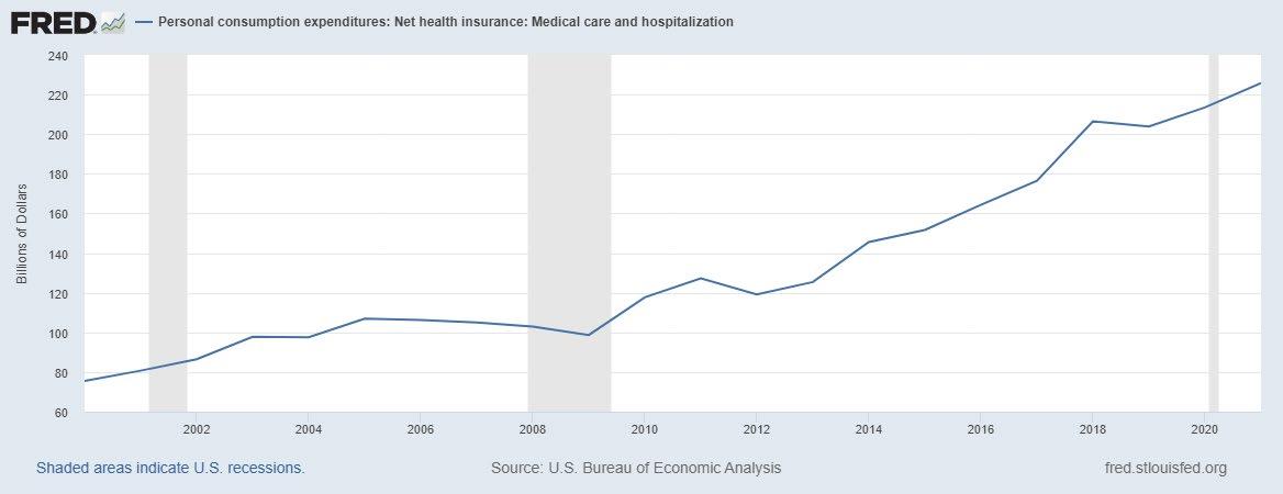
Source: St. Louis Federal Reserve, FRED
This exhibit represents current trends in Personal Consumption Expenditure on net health insurance. PCE represents the prices that individuals are paying for goods and services. The trend line shows are sharp increase in prices paid over the past 10 years on net health insurance. This may indicate an increase in the cost of healthcare.
121
3.0 LITERATURE REVIEW
The World Health Organization Commission on Social Determinants of Health identifies two main levels at which determinants operate. The first determinants are structural. Structural determinants are the fundamental structures that generate social stratification, such as global and national economic, political, and social welfare systems, and education systems. The second level is Proximal determinants. Proximal determinants are often called intermediate determinants as they are the circumstances of daily life. This includes the quality of family environment and peer relationships, through availability of food, housing, and recreation to access to education (Viner et al. 2012).
Poor social and economic circumstances affect individuals throughout their lives and people who are further down the social ladder are twice as likely to experience serious illness as well as premature death (Wilkinson & Marmot, 2003). Health care access is one of the major barriers that contribute to health disparities in the immigrant population. And as of 2017, there were still over 28 million people in the United States without health insurance. Since there are many difficulties of obtaining public health insurance, many immigrants rely on employer-based insurance or community health clinics to access medical care. Poverty is also a strong determinant of child well-being and is very common among immigrant children. (Orgera & Tolbert, 2020)
The most important factors that affect demand for medical insurance include household relative income and socio-economic status, household health status, people’s riskaversion intensity, and demographic factors (Kiil, 2012) Studies also examined determinants of health insurance enrollment in terms of socioeconomic factors. Sociodemographic factors, place of residence, behavioral factors, and household size. Income, employment, and wealth index are also very important factors. (Duku, 2018)
Cameron et al. examined the relationship between oncome and health and concluded that income predicts the purchase of health insurance. The higher the income, the less opportunity cost of purchasing health insurance (Cameron et al. 1988).
Kirgia et al. (2005) discuss that marital status has a significant positive impact on the demand for health insurance. Married couples demand more health insurance that unmarried couples are there are usually children who need protection and the avoidance of unaffordable health expenditures. Education may also increase people’s ability to
122
understand the benefits of risk management and even long-term savings, making education a determinant of health insurance consumption. (World Health Organization, 2007)
Greater national wealth improves health outcomes in children and adults and there is substantial evidence supporting that income inequality within countries affects various aspects of adolescent health, particularly within middle- and high-income countries. The World Health Organization Commission on Social Determinants of Health emphasized the evidence that educational attainment in early life with later health outcomes. Specifically, that improved education of women has a substantial benefit for the health of children worldwide. Sex inequalities are present in many aspects of health in adults in high-income countries. In adolescence, girls have poorer wellbeing indicators as selfrated health, psychosomatic complaints or symptoms, and life satisfaction, where boys have higher levels of injury and a greater likelihood of being overweight. Family factors are also a strong determinant of health. Families are the primary influence on the development of children. The WHO Commission on Social Determinants of Health identified supporting parents to improve early childhood development as a crucial step in the improvement of global health (The World Health Organization). adolescence is also a key period for the adoption of poor health behaviors. These behaviors can include substance misuse, unprotected sex, poor diet, lack of exercise, etc. These behaviors are shaped by social, economic, and cultural forces, and are major determinants of ill health across the course of life. (Viner et al. 2012)
4.0 DATA AND EMPIRICAL METHODOLOGY
4.1 Data
The data was obtained from the NYC.gov which is the official website of The City of New York. Under the health sector they offer information for individuals regarding birth certificates, death certificates, and vaccines. The department provides interactive tools as well as downloaded datasets. Some of these sets include community health surveys from 2002-2020. The dataset used in this study is the 2019 community
123
health survey containing 8,803 participants. The data was obtained through a series of questions over the phone.
Table 1: Summary Statistics
Dependent Variable Definition Mean Standard Deviation Insured Given a 1 if individual is insured. 0 if otherwise .8967 .3042 Independent Variables Race Race White Given a 1 if white. 0 if otherwise .3471 .4760 Race Black Given a 1 if black. 0 if otherwise .2207 .4147 Race Latinx Given a 1 if Latinx. 0 if otherwise .2738 .4459 Race Asian Given a 1 if Asian. 0 if otherwise .1280 .3341 Race Other Given a 1 if other. 0 if otherwise 0302 .1711 Employment Employed Given a 1 if employed. 0 if otherwise .5734 .4946 Unemployed Given a 1 if unemployed. 0 if otherwise .0627 .2424 Not in Labor Force Given a 1 if not in labor force. 0 if otherwise .3540 .4782 Education Less than High School Given a 1 if less than high school education. 0 if otherwise .1308 .3372 High School Graduate Given a 1 if graduated high school. 0 if otherwise .2020 .4015 Some College Given a 1 if attended some college. 0 if otherwise .2107 .4078 124
College Graduate Given a 1 if college graduate. 0 if otherwise .4516 .4976 Children Has Children Given a 1 if has children. 0 if otherwise .3359 .4723 Does not have Children Given a 1 if does not have children. 0 if otherwise .6594 .4739 Flu Vaccine Got Flu Vaccine Given a 1 if received flu vaccine. 0 if otherwise .5035 .5000 Did not get Flu Vaccine Given a 1 if did not get the flu vaccine. 0 if otherwise .4874 .4998 Marital Status Married Given a 1 if married. 0 if otherwise .3779 .4848 Divorced Given a 1 if divorced. 0 if otherwise. .1185 .3233 Widowed Given a 1 if widowed. 0 if otherwise .0842 .2778 Separated Given a 1 if separated. 0 if otherwise .0465 .2107 Never Married Given a 1 if never married. 0 if otherwise. .3013 .4588 125
Table 2: Race and Rates of Insurance
Table 3: Race and Sex and Rates and Insurance
Race Insured White 94% Black 89% Asian 90% Latinx 79% Other 87%
Race/Sex Insured White Female 95% White Male 94% Black Female 92% Asian Female 92% Asian Male 89% Other Male 89% Black Male 86% Latinx Female 85% Other Female 85% Latinx Male 74% 126
4.2 Empirical Model
Model 1 Insured = β0 + β1Female i
Model 2 Insured = β0 + β1Whitei + β2Blacki + β3Asianβi + β4Latinxi + β5Otheri + ε i
Model 3 Insured = β0 + β1Femalei + β2Whitei + β3Blacki + β4Latinxi + β5Asiani + β6Otheri + εi
Model 4 Insured = β0 + β1Whitei + β2Blacki + β3Latinxi + β4Asiani + β5Otheri β6EmploymentStatusi + β7Educationi + β8MartialStatusi + β9FluVaccinei + β10Childreni + εi
Model 1 focuses solely on the dependent variable, insured, and the relationship to the sex. In this model the omitted variable is male, so the model represents the relationship between females and insurance. Model 2 removes sex and accounts for the race variables White, Black, Asian, Latinx, and Other race individuals. The comparison variable in this model is Other race individuals. Model 3 adds sex back while also including the race variables, and again, Other race is the comparison. Lastly, Model 4 includes the race variables as well controlling for employment status, education, martial status, flue vaccine status, and if an individual has children. When all the models are analyzed, the individuals with the highest likelihood of insurance compared to Other race individuals will be determined, as well as determining whether controls vary results.
5.0 EMPIRICAL RESULTS
Variable Model 1 Model 2 Model 3 Model 4 Females .0406*** (.0065) .0466*** (.0064) 127
Table 4: Regression Results
Race White .0567** (.0200) .0563*** (.0199) .0338** (.0195) Race Black -.0085 (.0199) -.01228 (.0199) -.0057 (.0223) Race Asian -.0016 (.0209) -.0008 (.0208) .0032 (.0205) Race Latinx -.0793*** (.019) -.0826*** (.0194) -.0543** (.0191 Flu Vaccine Received Vaccine .0338 (.0329) Did not Receive Vaccine -.0190 (.0328) Has Children -.0386 (.05220 Does not have Children -.0377 (.0520) Employed .0322 (.0278) Unemployed .0110 (.0294) Not in Labor Force .1095*** (.0281) Less than High School .0658* (.0377) High School Graduate .1104*** (.0374) Some College .1384*** (.0375) College Graduate .1704*** (.0373) Married -.0298 (.0383) 128
The results of Model 1 yield significance at the 1% level between sex and insurance. As mentioned, males are the omitted category in this model. The marginal value of females is .0406. The positive value indicates that relative to men, women have an increased likelihood of insurance.
Model 2 removes sex while adding White, Black, Asian, Latinx, and Other (as the comparison variable). The model yields significance at the 5% level between White and Other, as well significance at the 1% level between Latinx and Other. The negative marginal value of Latinx (-.0793) represents that there is a decreased likelihood in insurance as compared to Other race. The positive marginal value of White indicates that there is an increased likelihood of insurance as compared to Other race individuals.
Model 3 includes sex as well as the race categories as well as Other race being the comparison variable.
Model 3 holds significance at the 1% level between Sex, specifically females. The positive marginal value of females holds as well indicating increased likelihood of insurance for females. The significance of the race White variable also holds at the 1% level as well as race Latinx. Identification as White shows an increased likelihood as compared to Other race, as represented by the positive marginal value. The negative marginal value of Latinx shows a decreased likelihood of insurance as compared to Other race.
Model 4, the last model, includes controls in the model. White and Latinx maintain significance at the 5%. White also holds its positive marginal value, concluding that controls aside, White individuals are at an increased likelihood of insurance. The negative
Divorced -.0359 (.0391) Widowed -.0017 (.0407) Separated -.0244 (.0407) Never Married -.0464 (.0383) Married Partner -.1012*** (.0393)
129
marginal value of Latinx concludes that controls aside, there is a decreased likelihood of insurance as compared to Other race individuals.
6.0 CONCLUSION
In summary, determinants of insurance are defined by two categories: structural & proximal. Structural determinants are the fundamental structures that generate social stratification, such as global and national economic, political, and social welfare systems, and education systems. Proximal determinants are often called intermediate determinants as they are the circumstances of daily life. This includes the quality of family environment and peer relationships, through availability of food, housing, and recreation to access to education. (Viner, et al. 2012) The most important factors that affect demand for medical insurance include household relative income and socio-economic status, household health status, people’s risk-aversion intensity, and demographic factors (Kiil, et al. 2012)
It can be concluded that women have a greater likelihood of insurance compared to men. White females have the highest rates of insurance while Latinx males have the lowest rates of insurance.
An important step to closing the healthcare gap is closing the Medicaid “coverage gap.”
The coverage gap includes more than 2 million adults that are mostly people of color. Many of these individuals have incomes below the poverty line but they live in states that refuse to adopt the Affordable Care Act’s Medicaid expansion. A long history of racially biased policy continues to remain as minority individuals are seen as undeserving of health services. Closing the gap of access to affordable healthcare is important to undoing the effects of structural racism that will continue to affect individual’s health. Medidacid expansion and subsidized private coverage through the ACA has reduced racial disparities in coverage but it must be consistent throughout the United States. (Harker, 2021)
130
Appendix A: Variable Description and Data Source
Acronym Description
Insured
If an individual has health insurance or not
Data Source
NYC Community Health Survey
RaceWhite Individuals who identify as White NYC Community Health Survey
RaceBlack Individuas who identify as Black.
NYC Community Health Survey
RaceAsian Individuals who identify as Asian NYC Community Health Survey
RaceLatinx Individuals who identify as Latinx
RaceOther Individuals who identify as another race
EmploymentStatus
MaritalStatus
Whether an individual is employed, unemployed, or not in the labor force
Whether an individual is married, divorced, widowed, separated, never married, married partner
NYC Community Health Survey
NYC Community Health Survey
NYC Community Health Survey
NYC Community Health Survey
FluVaccine
Children
EducationStatus
Whether someone received the flu vaccine or not
Whether an individual has children or not
Whether someone did not graduate high school, graduated high school, some college, college graduate.
NYC Community Health Survey
NYC Community Health Survey
NYC Community Health Survey
131
BIBLIOGRAPHY
Bhatt J, Bathija P. Ensuring Access to Quality Health Care in Vulnerable Communities. Acad Med. 2018 Sep;93(9):1271-1275. doi: 10.1097/ACM.0000000000002254. PMID: 29697433; PMCID: PMC6112847.
Cameron AC, Trivedi PK, Milne F, Piggott J. A micro-econometric model of the demand for health care and health insurance in Australia. Rev Econ Stud. 1988;55(1):85–106.
Duku S. (2018). Differences in the determinants of health insurance enrolment among workingage adults in two regions in Ghana. BMC health services research, 18(1), 384.
https://doi.org/10.1186/s12913-018-3192-9
Harker, L. (2021). Closing the Coverage Gap a Critical Step for Advancing Health and Economic Justice. Center on Budget and Policy Priorities.
Kiil A. What characterises the privately insured in universal health care systems? A review of the empirical evidence. [Epub 2012 Mar 27];Health Policy. 2012 106(1):60–75.
Kirigia J. M, Sambo L. G, Nganda B, Mwabu G. M, Chatora R, Mwase T. Determinants of health insurance ownership among South African women. BMC health services research. 2005;5(1):17.
Tolbert, J., & Orgera, K. (2020, November 12). Key facts about the uninsured population. KFF. Retrieved April 29, 2022, from https://www.kff.org/uninsured/issue-brief/key-factsabout-the-uninsured-population/
Romero, D., Echeverria, S. E., Duffy, M., Roberts, L., & Pozen, A. (2018). Development of a wellness trust to improve population health: Case-study of a United States urban center. Preventive medicine reports, 10, 292–298. https://doi.org/10.1016/j.pmedr.2018.03.009
U.S. Bureau of Economic Analysis, Personal consumption expenditures: Net health insurance: Medical care and hospitalization, retrieved from FRED, Federal Reserve Bank of St. Louis; https://fred.stlouisfed.org/series/DMINRC1A027NBEA, May 3, 2022.
Viner, R. M., Ozer, E. M., Denny, S., Marmot, M., Resnick, M., Fatusi, A., & Currie, C. (2012). Adolescence and the social determinants of health. Lancet (London, England), 379(9826), 1641–1652. https://doi.org/10.1016/S0140-6736(12)60149-4
Wilkinson, R.G. and Marmot, M.G. (2003) Social Determinants of Health: The Solid Facts: World Health Organization.
132
Wray CM, Khare M, Keyhani S. Access to Care, Cost of Care, and Satisfaction With Care
Among Adults With Private and Public Health Insurance in the US. JAMA Netw Open. 2021;4(6):e2110275. doi:10.1001/jamanetworkopen.2021.10275
World Health Organization. (n.d.). Social Determinants of Health. World Health Organization. Retrieved April 29, 2022, from https://www.who.int/health-topics/social-determinants-ofhealth#tab=tab_1
133
Panel Data Analysis: Gender Wage Gap and Macroeconomic Factors Impacts
Yuzhe Lin
Abstract:
This paper study the relationship between the gender wage gaps and macroeconomic factors that would impact them. The paper use panel data with data collected from OCED and World Bank WDI Indicator. The results show that the difference between female and male life expectancy, import, and female labor participation has a positive impact on the gender wage gap. FDI and Women business and law index score has a negative impact the gender wage gap.
JEL Classification: J16, F4, F43
Key Word: Gender wage gap, panel data
134
The difference between gender is a topic that has been discussed a lot more recently year. There are lots of ways that two gender are treated differently. For example, females tend to have a lower degree than males in lots of countries. Different countries have different customs that lead to the result. For example, in China, back in old times, as a female married a male, their children only go with the last name of the male instead of the female, so that the family of the female would lose their inheritance as their family is not inherited. As a result, women are less likely to be supported to go to school. Also, since males are believed to be more intelligent than females, families tend to support male than females.
Although the discrimination against females is getting awareness by the government, there are still things that could be understood as unbalance between females and males in their working field. One of the examples would be the “motherhood penalty”. It is the negative effects of childbirth on a mother’s employment and wages as they need to have enough rest both before and after giving birth. The research paper by Yu-Wei Luke et al. (2020) discusses its effects and comes to a conclusion that childbearing on mothers’ labor supply is less negative in countries with smaller gender wage gaps and declines in a country’s gender wage gap is strongly associated with reductions in the motherhood employment penalty.
In this paper, we are focusing on the impact of openness of the country has been presented as the import per year, the difference between the life expectancy of males and females, the gross domestic product (GDP) growth, the women's business and law index score, Foreign direct investment(FDI), and female labor force participation rate to the gender wage gap with data from 11 countries from the year 2000 to 2019. We expected that the openness of the country would have a positive impact on the gender wage gap that is the higher the openness of a country, the lower the gender wage gap would be. As a country is more open, the people would tend to have a better idea of the gender wage gap so that it would diminish. The women's business and law index score is the knowledge and analysis provided by Women, Business and the Law make a strong economic case for laws that empower women. Better performance in the areas measured by the Women, Business, and the Law index is associated with more women in the labor force and with higher income, and improved development outcomes. Equality before the law and economic opportunity is not only wise social policy but also good economic policy. The equal
1.0 INTRODUCTION:
135
participation of women and men will give every economy a chance to achieve its potential. Life expectancy is the data that on average, how long would a male or female would live, we believe it is important as it reflects how males and females are treated in that country. The FDI is the measurement of how the foreign investor invests in the country and can be seen as a factor in how open a country is. The female labor force participation rate is a factor that reflects how female labor is treated in the country and should have a positive relationship with the gender wage gap as a lower gender wage gap should lead to a lower female labor participation rate.
2.0
Figure 1 shows the gender wage gap in 11 countries from 2000 to 2019 (Country1=Japan, 2=USA,3=UK,4=AUS,5=AUT,6=BEL,7=CAN,8=CZE, 9=DEU, 10=FIN,11=HUN). From the graph, it can be seen that the gender wage gap in most countries is getting lower, it is a good sign to be seen as the gender wage gap is a type of discrimination against females. Figure 2 gives an overview of the Women’s business and law index from the year 2000 to 2019.
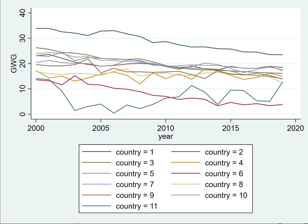
Figure
Source: OECD
Trend:
Figure 1: Gender wage gap in 11 countries from 2000 to 2019
136
2: Women’s Business and Law Index from 2000 to 2019
Source: World Bank Database
Source: World Bank Database
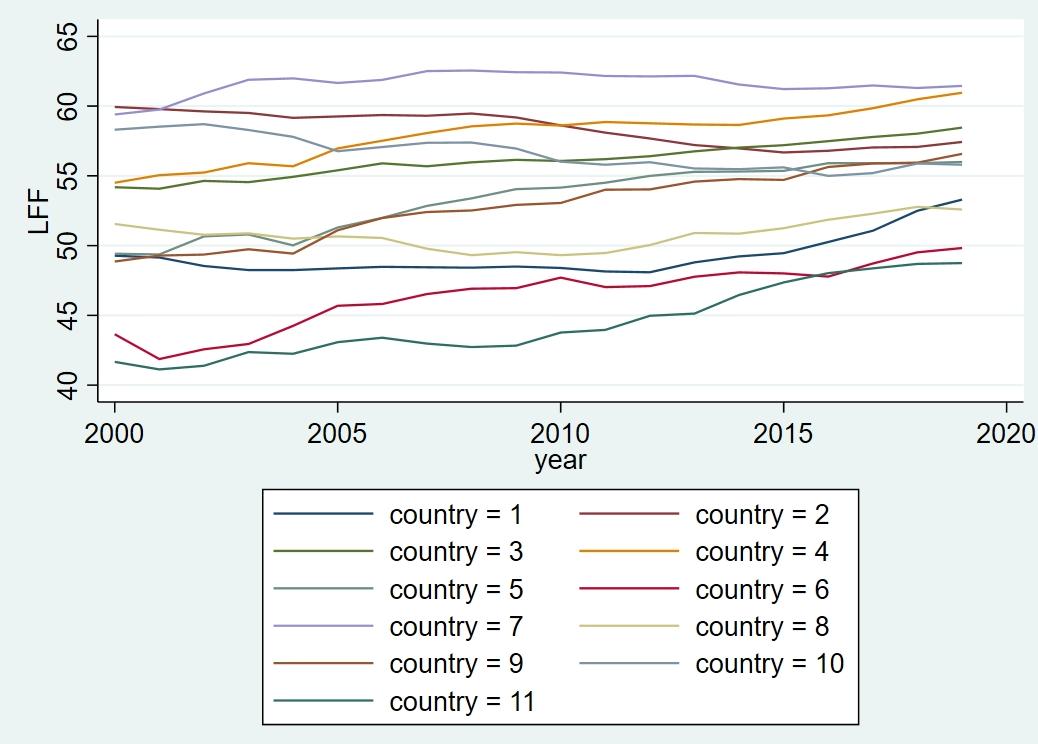
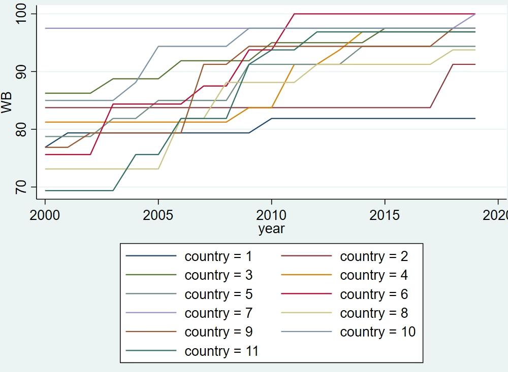 Figure 3: female labor force participation rate from 2000 to 2019
137
Audi et al. (2017) conduct research about the relationship between the openness of the society (trade liberalization) of SAARC countries and the gender gap. From their model, they find that the relationship between female unemployment rates with GDI is insignificant but negative, when the gross domestic product is increasing, the gender gap (female to male labor participation rate) will go down. And the relationship between GDP growth and the female-tomale participation rate is positive and significant which means growth in the economy encourages the participation of females in the labor market which reduces the gender gap.
Vaccaro et al. (2022) study the gender wage gap in Peru and its relationship with education. Their model shows the result that education in the unexplained and explained component contributes to reducing the observable gap between working men and women. And the GDP per capita is negatively correlated with the gender wage gap.
Seguino (2000) discusses the relationship between gender inequality and GDP growth rate by using panel data for analysis. They concluded that gender wage inequality and growth are positively correlated with each other which is different than the result of Audi et al. (2017).
Mussida and Picchio (2012) discuss the relationship between the gender wage gap and education in Italy. They find that female employees who have lower education level tend to receive more wage penalty than female employees who has higher education level. Mussida and Picchio conclude that “First, if men and women had the same characteristics women would suffer significant and large pay penalties, independently on whether we correct for nonrandom selection into full-time employment and on educational levels. Second, low educated women suffer much larger pay penalties, especially after correcting for sample selection and at the bottom of the wage distribution.” (2012)
Seguino(1997)investigates the relationship between gender, wage inequality, and export growth in South Korea. The study shows different results than previous studies as the study shows that gender inequality does not contribute to export-oriented growth strategy, and the reason may be because the particular country the author chose may not apply to other markets.
3.0 Literature Review:
138
Stokke (2021) studies the gender wage gap and how its education and real experience impact it. And the study shows that the gender wage gap uses the potential rather than actual, real experience. And higher education workers would receive more which is reasonable.
Langdon and Klomegah (2013) study more generally the gender wage and factors that impact it, such as occupation, education, and traditional gender ideology. They come to the conclusion that there are lots of important factors that impact the gender wage gap, occupation, education, race, age, and gender ideology all have a significant impact on it. And gender ideology is the most important factor in their study.
4.0 Data and Empirical Methodology
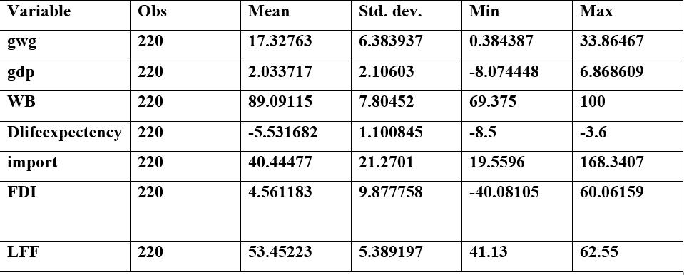
4.1 Data
The study uses gender wage gap data from OECD and other variables gathered from World bank Database for twelve countries within the period 2000 to 2019. The countries are picked from different Continents including Asia, Euro, and North America.
GWG=GWG=α+β1*GDP+β2*WB+β3*life+β4*import+β5*FDI+β6*LFF+γ
GWG: gender wage gap (%)
Table 1: Data Summary
4.2 Empirical Model Model
139
GDP: GDP growth (annual %)
IMPORT: import (% of GDP)
Dlifeexpectency: male life expectancy -female life expectancy
WB: women business
FDI: foreign direct investment
5.0 Empirical Results
5.1 Conclusion
In summary, from the result of the regression, the difference between life expectancy, import, and female labor participation has a positive impact on the gender wage gap. FDI and Women's business and law index score has a negative impact on the gender wage gap. The GDP impact is not statistically significant.
The study discusses the impact of macroeconomic factors on the gender wage gap. There are lots of limitations of the study, first, the data set is not large enough as there are not enough data included in the data set, only 11 countries with 20 years range of data are included, the more data included in the study, the better the prediction of the result could be. The government could pay more attention to the law and regulations that help females build their carrier, from the study, the WB is negatively related to the gender wage gap which may show that the laws and regulations are not enough to help females with their carrier.
Variable Coefficient Std. err. P value gdp .1199456 .0827238 0.149 import -.1113024** .0516457 0.032 WB .0957646* .0511191 0.062 life -2.754769*** .6039036 0.000 FDI .0309553* .017376 0.076 LFF -.2758755** .1263987 0.030
Table 2: Result Table
140
Bibliography
Hussain, M. A., & ., A. A. (2018). Gender gap and trade liberalization: An analysis of some selected SAARC countries. Advances in Social Sciences Research Journal, 5(11).
Langdon, D. L., & Klomegah, R. (2013). Gender wage gap and its associated factors: an examination of traditional gender ideology, education, and occupation. International Review of Modern Sociology, 39(2), 173–203.
Mussida, C., & Picchio, M. (2012). The gender wage gap by education in Italy. SSRN Electronic Journal.
Chu, Y.-W. L., Cuffe, H. E., & Doan, N. (2020). Motherhood Employment Penalty and Gender Wage Gap across countries: 1990–2010. SSRN Electronic Journal
Seguino, S. (1997). Gender wage inequality and export‐led growth in South Korea. The Journal of Development Studies, 34(2), 102–132.
Seguino, S. (2000). Gender inequality and economic growth: A cross-country analysis. World Development, 28(7), 1211–1230.
Vaccaro, G., Basurto, M. P., Beltrán, A., & Montoya, M. (2022). The gender wage gap in Peru: Drivers, evolution, and heterogeneities. Social Inclusion, 10(1), 19–34.
Woetzel, J., Madgavkar, A., Ellingrud, K., Labaye, E., Devillard, S., Kutcher, E., Manyika, J., Dobbs, R., & Krishnan, M. (2020, September 16). How advancing women's equality can add $12 trillion to global growth. McKinsey & Company. Retrieved March 19, 2022.
Stokke, H. E. (2021). The gender wage gap and the early‐career effect: The role of actual experience and education level. LABOUR, 35(2), 135–162.
141
The Effect of Minimum Wage Increases on Employment of Teenagers in New England
Felicia O’Reillya
Abstract:
This paper examines the relationship between increasing minimum wage and the number of hours that teenagers ages 15-19 work in New England states during the years 20022019. In these years, all New England states have had various minimum wage rates, this paper will use feasible general least squares state-level panel data analysis to see if there is a positive or negative impact on teenage employment due to increases in minimum wage. Data was collected from the Current Population Survey, the American Community Survey, and state census data, and used with an equation derived by Zavodny (2000).
State-level panel data analysis for Maine, New Hampshire, Vermont, Massachusetts, Connecticut, and Rhode Island was performed and regression results showed that minimum wage has a negative impact on teen employment in New England.
JEL Classification: J21, J31, J38, J81.
Keywords: Minimum wage, Unemployment, Hours, Teenagers.
a Bryant University, 1150 Douglas Pike, Smithfield, RI02917. Phone: (207) 756-5591.
Email: foreilly@bryant.edu.
142
Minimum wage has been changing in the United States ever since it was established in 1938 with the passing of the Fair Labor Standards Act. The federal minimum wage continues to spark debate across the US as it does not adjust to the rising standards of living. The purpose of minimum wage is to protect workers against being paid too little for their labor. The minimum wage applies to those at the lower end of the wage distribution in the United States. Since it was first instituted, the federal minimum wage has been raised over 22 times. States however are able to set their own minimum wage higher than the federal minimum wage, but not lower than the federal rate. Massachusetts was the first state to enact a minimum wage back in 1912 and other states followed suit. Since minimum wages are defined nominally, “their purchasing power shrinks with inflation,” meaning that employees living off of minimum wage jobs are struggling to keep up with the current standard of living (Simonovits et. al, 2019). Those working minimum wage jobs are more likely to support increasing the minimum wage because they will be the ones reaping the benefits.
Minimum wage has contributed to closing the wage gap in various countries as being a building block for workers to learn valuable skills that they can use when they move up to higher paying jobs. Teen employment on the other hand has been declining for the past few decades as less and less teens are interested in getting a job. There are also more teens who are in school during the summer or opt for community service ventures as a way to add more to their college resumes. Teens are also interested in doing internships, many of which are unpaid which the Current Population Survey does not count as being employed. Financial aid opportunities have also increased over recent years which means having a job is not as important to teenagers to fund their college tuition because they have other options. There has been limited research into the effect changes in minimum wage has on teen employment in the United States. Teen employment declines during the business cycle but hypothetically, raising the minimum wage should encourage more teens to work, but research has shown that it has the opposite effect. Instead of opting for more work and taking advantage of the pay increase, many teens choose to work less when minimum wage is increased. It is important to examine the full effects of minimum wage
1.0 INTRODUCTION
143
to understand why it has the effects on minimum wage that it does. This paper was guided by three research objectives that differ from other studies: First, it focuses specifically on the 6 New England states from 2002-2019, rather than all 50 states over an extended period of time, in order to get a closer look into the effects of minimum wage. Second, it will utilize feasible general least squares regression analysis rather than fixed effects and random effects in order to account for heteroskedasticity and serial correlation amongst the data. Lastly, it will aim to understand the full effects that increasing state minimum wages has had on teen employment over the years.
The rest of the paper is organized as follows: Section 2 shows some background on the trends of minimum wage in the United States over the past decades. Section 3 gives a brief literature review. Section 4 outlines the data and empirical methodology used. Section 5 presents and discusses the empirical results. Section 6 will discuss the limitations of this study. This is followed by a conclusion in section 7.
2.0 HISTORICAL CHANGES IN MINIMUM WAGE
Figure 1 shows the changes in the federal minimum wage in the United States since 1968. The first federal minimum wage enacted under the Federal Fair Labor Standards Act was $0.25/hour. Since then, the federal minimum wage was enacted, it has steadily increased. It peaked in 2010 at $7.25/hour and since 2010, it has remained constant through 2021, but many states have enacted minimum wages above the set federal minimum wage. While some argue that raising minimum wage would raise the earnings of most low-income workers, the government tries to set the minimum wage at a rate that would not cause low-wage workers to become jobless due to companies not being able to afford their workers.
144
Figure 1: Federal Minimum Wage Rate under the Federal Fair Labor Standards Act
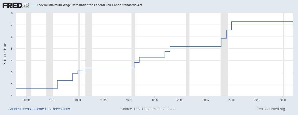
Figure 2 shows states with minimum wages set above the mandated federal minimum wage as of January 1, 2022. The grey states represent states which match the federally mandated minimum wage while the blue represents states that have set their minimum wages above the federal minimum wage. The darker blue states have the highest state minimum wages however the lighter blue states still have minimum wages set over $7.25/hour. Many states have historically set their minimum wages above the federal minimum wage while others have opted to maintain the federal minimum wage.
All 6 New England states except for New Hampshire have state minimum wages above the federal minimum wage rate.
Source: St. Louis FRED (Federal Reserve Bank of St. Louis)
145
The Economic Policy Institute defines bound states as states with minimum wages less than $6.55 in January 2008. Unbound states have minimum wages greater than $6.55 in January 2008. During the Great Recession that hit in late 2007, many blamed the federal minimum wage increase for workers losing their jobs, but the Economic Policy Institute argues that the recession itself is to blame for the loss of jobs, rather than because of the increase in minimum wage as Figure 3 shows.
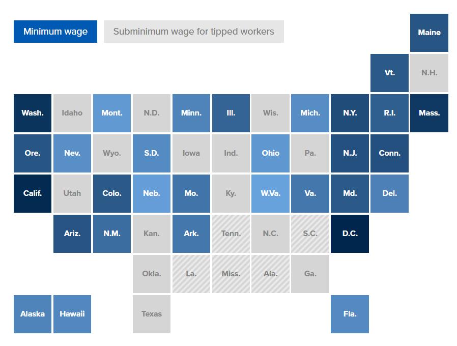 Figure 2: States with Minimum Wage above Federal Minimum Wage as of 2022
Source: Economic Policy Institute
Figure 2: States with Minimum Wage above Federal Minimum Wage as of 2022
Source: Economic Policy Institute
146
3.0 LITERATURE REVIEW
The effects of minimum wage have been a topic of interest for economists ever since its introduction in 1938. There has been large debate for years over whether or not raising the minimum wage would help to close the wage gap by encouraging more people to work. Minimum wage jobs are traditionally held by teenagers as it is normally their first jobs and all that they are qualified for. Since minimum wage jobs are normally starter jobs, meaning it is where workers learn skills in order to move up, they are necessary jobs in the economy. Historical research has shown that typically, minimum wage increases result in a fall in employment as employers hire less so that they do not have to pay as many workers. Larger companies are more equipped to handle minimum
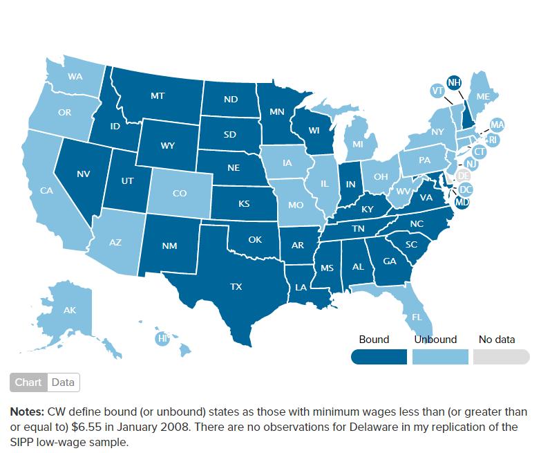 Figure 3: Bound and Unbound States after the Federal Minimum Wage Increase in 2007
Source: Economic Policy Institute
Figure 3: Bound and Unbound States after the Federal Minimum Wage Increase in 2007
Source: Economic Policy Institute
147
wage increases because they have more money available to pay wages than smaller companies. The smaller companies take a bigger hit from minimum wage increases because they cannot afford to give all of their minimum wage workers raises.
According to the Federal Fair Labor Standards Act, states are allowed to set their own minimum wages as long as the state mandated wage is equal to or greater than the federal minimum wage. Simonovits et. al (2019) researched how public opinion influences state and federal legislation in the United States. Most voters in Simonovits et. al’s (2019) study prefer their state minimum wage to be higher than what it is currently set at. While direct democracy institutions may increase representation in enacted policies regarding minimum wage, individual bias still exists which can derail the process entirely. Many constituents have come to the realization that changing minimum wage is more possible at a local level than it is at a national level. As of 2018, Washington had a statewide minimum wage of $12/hour while the federal minimum wage remained at $7.25/hour. Seattle, Washington however, required large businesses in the city to pay their employees at least $15/hour. As raising minimum wage is a primarily liberal agenda, local areas are able to change their minimum wage laws without pushing that agenda on other parts of the state where voters may disagree with the policy.
The previous research on how minimum wage affects teen employment has mostly focused on all 50 states over a broad number of years In her paper, Madeline Zavodny (2000) looked at state-level and individual-level panel data to examine the effects of rising minimum wage on teen employment The state-level analysis she conducted showed that while minimum wage increases may lower unemployment rates, it “does not adversely affect hours among either working teens or all teens” (Zavodny, 2000). When minimum wage is raised, firms must find alternative ways to save money if they do not want to fire any of their workers. Some employers choose to reduce the hours of their employees when there is an increase in minimum wage. They also rely on their employees wanting to work less because of their increase in income. Zavodny (2000) found that while minimum wage increases can have negative employment effects, it does not appear to decrease hours of work.
Giuliano (2013) focused on minimum wage effects on the teen labor supply within a large US retail firm; she found that in response to the 1996 federal minimum
148
wage increase, employment of teenagers increased significantly. She found that if minimum wage is not set too high, it can benefit low-wage workers by “raising both their wages and employment levels” (Guiliano, 2013). The retail sector accounts for many teenage workers in the US so Guiliano’s (2013) research is a good indicator for how minimum wage affects teen employment in the US. While her research showed that compulsory increases in the average wage did not show significant effects on boosting unemployment, teenage workers do not respond the same as the public as a whole when it comes to increases in the minimum wage (Guiliano, 2013). In her findings, Guiliano (2013) found that in markets with lower initial wages to begin with, an increase in minimum wage affected the wages of both adults and teenagers, however it mostly affected adults. In higher-wage markets, minimum wage increases mainly affected the wages of teenagers and had a positive affect on teenage employment in general (Guiliano, 2013). However, she posits that the increases in minimum wage benefit the teen employment the most when there are small increases only and that large increases could have the opposite effect (Giuliano, 2013).
Kalenkoski and Lacombe (2013) looked specifically at how minimum wage increases affect teen employment when employment is correlated across political boundaries. When minimum wage is increased in one state, that often means that employees in neighboring states will cross the state border in order to gain access to higher wages. By using a spatial econometrics approach, Kalenkoski and Lacombe (2013), found that a 10% increase in minimum wage led to about a 2% decrease in teen employment. Kalenkoski and Lacombe (2013) found that most economists researching this type of data used a relative wage rather than the real effective minimum wage. Zavodny (2000) however, argues that using the real minimum wage instead of the average adult minimum wage is imperative because the average adult minimum wage is correlated with business cycle conditions. This means that the effects of business cycle conditions on teen employment would be included when the focus should be on how minimum wage increases affect teen employment.
Cengiz et. al (2019) opted to use a difference-in-differences approach to examine the effect of minimum wages on low-wage jobs using state-level minimum wage changes from 1979 to 2016. In their research on the effects of minimum wage, Cengiz et. al
149
(2019) found that there has been little research on the effect of minimum wage policies on overall employment. By focusing on the effects of minimum wage on the frequency distribution of wages in the U.S., Cengiz et. al (2019) found that “an average minimum wage hike led to a significant decrease in the number of jobs below the new minimum wage in the five years after implementation.”
Labor force participation for teenagers has been on the decline for many years. There are various reasons for this, many parents do not want their teenage children working during the school year because they want them to focus on their studies. Neumark and Shupe (2019) found that the labor force participation rate of teenagers ages 16-19 fell from 52.7% in 1994, to 43.9% in 2004, and to 34.0% in 2014. Raising minimum wages can reduce employment opportunities for young workers as there are less jobs available. As more low-skilled immigrants come to the U.S., there is also more competition for minimum wage jobs which may discourage teenagers from working. Another reason for teen employment declining that Neumark and Shupe (2019) found is that there are higher returns to schooling, meaning that when minimum wage goes up, often times there is an increase in investment in schooling.
4.0 DATA AND EMPIRICAL METHODOLOGY
4.1 Data
The study uses annual data with a panel data analysis of all 6 New England states for the years 2002-2019. Data were obtained from the Current Population Survey, the American Community Survey, and state census data Using these numbers, averages were calculated in Excel from equations provided by Zavodny (2000). Fixed effects, random effects, and OLS regression analysis were conducted, and after examining those results, feasible general least squares panel data was conducted to control for heteroskedasticity and auto correlation (AR1) or serial correlation.
Summary statistics for the data are provided in Table 1.
150
Table 1 Summary Statistics
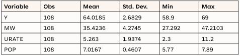
4.2 Empirical Model
This paper uses Zavodny’s (2000) model which she used to analyze the minimum wage effects on all 50 states. This study adapts on Zavodny’s (2000) original research and specifically examines the data for New England states instead of all 50 states in the years 2002-2019, which will be all years after Zavodny did her research
The model could be written as follow:
Yit is the dependent variable and is the employment to population ratio, average weekly hours of all teens, or average weekly hours of employed teens in state i in year t ; in this case, the teen employment to population ratio was used as a measure for teen employment. There are five independent variables used. MWit is the minimum wage variable and it can be measured by the effective minimum wage deflated using the personal consumption expenditures (PCE) index or the relative minimum wage (the minimum wage divided by average adult hourly earnings). In this case, MWit is measured by the relative minimum wage by state. URATEit is the unemployment rate per state.
δPOPit is the ratio of teens aged 15-19 to the total population. Si and Tt are state and year fixed effects to control for time-invariant unobservable differences across states and business-cycle effects common to all states. Appendixes A and B provide data sources, acronyms, descriptions, and expected signs for using the variables.
lnYit = α + βlnMWit + γURATEit + δPOPit + + σSi + θTt + εit (1)
151
5.0 EMPIRICAL RESULTS
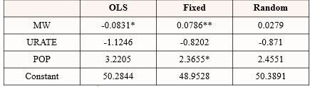
The empirical estimation results are presented in Table 2 and Table 3, along with the correlation matrix in Table 4. Fixed effects, random effects, and OLS regressions were all conducted in order to figure out which type of regression was best. Due to heteroskedasticity and AR1 correlation, feasible general least squares state-level panel data analysis was performed, and those results showed that consistent with past research such as Zavodny (2000) and Kalenkoski & Lacombe (2011), state minimum wage increases results in a decrease in teen employment.
In Zavodny’s (2000) original research, she opted not to perform these types of regressions because of the type of data being analyzed. Though there was some 5% and 10% significance in the OLS, fixed effects, and random effects regression analyses, these regressions did not fit this type of data. Due to AR1 correlation and heteroskedasticity in the data, the probability F test showed that prob > F was equal to 0. While some believe that this means the data is very significant, having the probability F test equaling 0 means that either the data is flawed, or the wrong regression analysis is being performed. Just as Zavodny (2000) used feasible general least squares analysis for her research, FGLS was the best fit regression analysis for this data. Table 2 shows the results of the fixed effects, random effects and OLS regression below.
Note: *** , **, and * denotes significance at the 1%, 5%, and 10% respectively.
The MW variable estimate was significant at the 5% level and showed that minimum wage has a negative effect on Y, the teen employment to population ratio for New England states. This was expected due to the results of past research and is
Table 2: Multiple Regression Results for New England
152
consistent with Zavodny’s (2000) research into the effect of minimum wage on teen employment. Her research looked at all 50 states and represents a more in-depth approach to analyzing the effects of minimum wage increases on teen employment. The URATE variable estimate was expected to have a negative impact on teen employment because as unemployment goes up, clearly employment must be going down. While the URATE had a negative effect on teen employment, it did not have any level of significance in the feasible general least squares regression. The POP variable estimate showed a 5% level of significance and FGLS regression results showed that an increase in the teen to total population ratio resulted in an increase in teen employment in New England states. These results were consistent with the research of Neumark & Shupe (2019) and Zavodny (2000). Table 3 shows the results of the FGLS regression analysis below.
Table 3: FGLS Regression Results for New England
Note: *** , **, and * denotes significance at the 1%, 5%, and 10% respectively
Table 4 shows the correlation matrix for Y, the measure for teen employment, MW, the minimum wage estimate, URATE, the unemployment rate, and POP, the teen to total population ratio. As expected, the URATE variable has a negative correlation with Y, a relationship which is expressed in the feasible general least squares regression analysis. POP, has a positive correlation with Y, teen employment, and this positive relationship is also expressed in the results of the FGLS regression analysis. MW, however, is shown to have a slight positive correlation with teen employment, Y. This is not represented through the results of the FGLS regression analysis. This has a simple explanation, the signs are opposite in the correlation matrix and the FGLS regression analysis because the original relationship between minimum wage, MW, and teen

153
employment, Y, is so close to zero, that the difference in signs reflects random variation around zero. Table 4 shows the correlation matrix below.
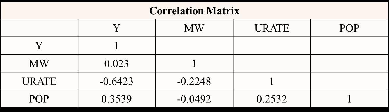
6.0 LIMITATIONS
This study only looks at 6 out of the 50 states making it a relatively small sample. In order to get more in-depth results, it would be better to look at all 50 states in order to understand the full effects that raising state minimum wages has on the entire country. It would also be better to look at more years of data, since this research only examined the years 2002-2019, it does not cover the full history of effects that minimum wage has had on New England states. It would also be interesting for future research to focus on one specific state’s full history to see if there are any discrepancies amongst the past research. It would also be beneficial for future research to add more variables to the equation to explore what else affects teen employment not only in New England states but in all of the states.
7.0 CONCLUSION
Overall, after conducting feasible general least squares state-level panel data analysis on all 6 New England states for the years 2002-2019, increasing state minimum wages was found to have a negative impact on teen employment in Connecticut, Maine, Massachusetts, New Hampshire, Rhode Island, and Vermont. Increasing unemployment rates was shown to have negative effects on teen employment in New England, while increasing teen to population ratio was found to have a positive effect on teen employment. Increasing minimum wage is not solely responsible for the declining teen
Table 4: Correlation Matrix
154
employment that the United States has seen over the years. As Neumark & Shupe (2019) report, though raising minimum wage can reduce employment opportunities for teenagers, the United States has also seen an increase in the number of low-skilled immigrants which has caused more competition for jobs typically held by teenagers who are also low-skilled. Teens are also seeing higher returns to schooling which has caused more parents to encourage their children to spend more time in school and less time working a part-time job.
155
Appendix A: Variable Description and Data Source
Acronym Description
Y Teen Employment: Teen to total employment ratio
MW Relative minimum wage: measured by dividing the state minimum wage by average adult hourly earnings
URATE State Unemployment Rate (respectively)
Data source
Current Population Survey
American Community Survey/state census data
POP Ratio of teens aged 15-19 to the total population
Current Population Survey
American Community Survey
S State Fixed Effects
T Year Fixed Effects
New England States
Years 2002-2019
156
Appendix B: Variables and Expected Signs
Acronym Variable Description What
MW Relative minimum wage: measured by dividing the state minimum wage by average adult hourly earnings
URATE State Unemployment Rate (respectively)
POP Ratio of teens aged 15-19 to the total population
Relative Minimum Wage by State -
Unemployment Rate by State -
Teen Population Ratio +
it captures Expected sign
157
BIBLIOGRAPHY
Cengiz, D., Dube, A., Lindner, A., & Zipperer, B. (2019). The effect of minimum wages on lowwage jobs. The Quarterly Journal of Economics, 134(3), 1405-1454.
David, H., Manning, A., & Smith, C. L. (2016). The contribution of the minimum wage to US wage inequality over three decades: a reassessment. American Economic Journal: Applied Economics, 8(1), 58-99.
Giuliano, L. (2013). Minimum wage effects on employment, substitution, and the teenage labor supply: Evidence from personnel data. Journal of Labor Economics, 31(1), 155-194.
Kalenkoski, C. M., & Lacombe, D. J. (2013). Minimum wages and teen employment: A spatial panel approach. Papers in Regional Science, 92(2), 407-417.
Lee, D. S. (1999). Wage inequality in the US during the 1980s: Rising dispersion or falling minimum wage?. Industrial Relations Section, Princeton University.
Li, S., & Ma, X. (2015). Impact of minimum wage on gender wage gaps in urban China. IZA Journal of Labor & Development, 4(1), 1-22.
Neumark, D., & Shupe, C. (2019). Declining teen employment: minimum wages, returns to schooling, and immigration. Labour Economics, 59, 49-68.
Sen, A., Rybczynski, K., & Van De Waal, C. (2011). Teen employment, poverty, and the minimum wage: Evidence from Canada. Labour Economics, 18(1), 36-47.
Simonovits, G., Guess, A. M., & Nagler, J. (2019). Responsiveness without representation: Evidence from minimum wage laws in US states. American Journal of Political Science, 63(2), 401-410.
Zavodny, M. (2000). The effect of the minimum wage on employment and hours. Labour Economics, 7(6), 729-750.
158
Panel Data Analysis of Import Tariff Policy on Economic Growth and Industrial Output in Developing Economies.
Connor A. Palazzo Bryant University
Email: cpalazzo1@bryant.edu
May, 2022.
Abstract
This paper is focused on interpreting the effects of import tariff policy on domestic economic growth in the small market economies of developing nations. There have been several previous studies that have investigated the effect of tariff policy on domestic consumers and producers of already established economies. In addition, there have also been many studies assessing the effects tariffs from developed countries have on developing countries. However, few reports have been done on how tariffs impact the domestic producers of a developing nation. It is widely accepted that open and free trade is the best method for facilitating growth and innovation across highly developed economies. However, for non-developed economies there is still a case to be made that tariff rather than free trade offer the most benefit. The argument made is that by protecting domestic firms from foreign competition, they can grow to a level that can compete with the large firms of developed economies.
Key Terms: Trade Policy, Economic Development, Tariffs, Import-Export, Economic Growth, Industrial Output
159
1.0 INTRODUCTION
This paper is focused on interpreting the effects of import tariff policy on domestic economic growth in the small market economies of developing nations. There have been several previous studies that have investigated the effect of tariff policy on domestic consumers and producers of already established economies. In addition, there have also been many studies assessing the effects tariffs from developed countries have on developing countries. However, few reports been done on how tariffs impact the domestic producers of a developing nation.
It is widely accepted that open and free trade is the best method for facilitating growth and innovation across highly developed economies. However, for non-developed economies there is still a case to be made that tariffs rather than free trade offer the most benefit. The case to be made is that by protecting domestic firms from foreign competition, they can grow to a level that can compete with the large firms of developed economies. Like America in the early-mid 19th century, developing countries rely primarily on agricultural and natural resources exports as their main source of income generation. However, growth of domestic industry and investment is crucial for reducing poverty, while creating the skilled job opportunities necessary for a middle class. A contrary argument can still be made that tariffs by restricting the access domestic firms have reaching foreign markets hinders growth. There is also the argument to be made that tariffs, by reducing competition and taxing foreign goods, increases inflation and negatively impacts consumers. This paper seeks to discover the relationship between tariff and growth focusing on 7 developing sub-Saharan African countries and to see if tariffs do support domestic firms in infant economies.
This study has been broken down into 7 sections. The section immediately following the introduction is the 2nd section and discusses the trends of tariffs and growth over the past few decades. Section 3 is the literature review which goes over the previous research that has been done by other researchers on similar topics regarding tariffs. Section 4 discusses the data used in this study and Section 5 goes over the regression models run. Section 6 goes over the regression results and finally Section 7 is the conclusion to this paper.
160
2.0 TREND
Figure 1 shows the trend of tariff rates from 1989 to 2008 of countries by income level. Countries are divided into four income groups. Tariff rates for all income groups have decreased but rates from lower-middle income countries have decreased the most, from near 25% on average to about 10%. High income countries have decreased their tariffs the least as they have consistently been low, less than 10% since 1989. Generally, we can observe that high-income countries have the lowest average tariff rate while low-income countries have the highest. A large reason for decreasing tariffs has to do with increased amounts of Preferential Trade Agreements (PTA) and the expansion of the World Trade Organization (WTO).
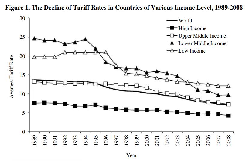
161
Source: Kwon, 2013.
3.0 LITERATURE REVIEW
Tariff policy and protectionism has been around for centuries around the world and for many decades in the mid-late 1800’s and early 1900’s, tariff policy was a stand-in for good foreign policy. However, after World War II a stance of trade liberalization and world governance combined with large economic growth around the world swung the conventional view of tariffs from one side to the other. Still there is disagreement among economists on the relationship between tariff implementation and a country’s economic growth (Baldwin, 2004). As Kwon (2013) suggests, this discrepancy of a strong positive relationship between tariffs and growth in the early 20th century combined with the negative relationship between tariffs and growth in the late 20th century, makes finding that true effects of tariffs on growth difficult and confusing. Baldwin (2004) points out that this is due to how broadly a researcher defines openness and this greatly effects the conclusion the researcher can draw. Baldwin’s conclusions from his study is that most studies find a strong positive relationship between “outward-looking” policies and growth and that empirical studies have demonstrated a positive casual connection between openness and economic growth. He points out that the implications of the findings suggest that governments should reduce their tariff levels but also insists that the evidence does support any claims that by reducing tariffs a country will necessarily see increased economic growth as a result.
Cheong et al. (2017) also looked at openness and growth by looking at the effectiveness of Preferential Trade Agreements (PTA) that countries sign. PTA’s are designed to primarily reduce tariffs and increase trade between countries and since the 1990’s the number of PTA’s in effect have increased dramatically (Cheong et al., 2017). Cheong et al. (2017) found that PTA’s have a significant positive effect on trade flows and forming a Free Trade Agreement (FTA) can increase trade flows by 6% to 22%. The conclusion of their results suggest that PTA’s do exactly what they are designed to do which is to increased trade. However, with this finding they show that tariffs also do what they are designed to do. Cheong et al. (2017) found that a 1% increase in prices due to tariff hikes can result in a deduction of 2.3% in bilateral trade flows. In other words, tariffs which are designed to reduce foreign competition do exactly that. The findings of Cheong et al. (2017) are supported by the finds of Edwards (1997) who examined openness, productivity, and growth in 93 countries and found that countries that are more open tended to experience much faster growth than closed countries.
162
From studies like the ones above there has developed a widely adopted belief that trade liberalization is the only way that developing countries can induce economic growth (Kwon, 2013). However, Kwon (2013) finds that tariffs and growth relationships may be contingent on other factors in conjunction with tariffs. This is consistent with the thoughts of Baldwin (2004) who found that tariffs and non-tariff barriers are often insignificant on their own. Indeed Kwon (2013) found that higher tariffs when combined with domestic investment and labor, results in higher economic growth according to his regression analysis.
This study follows the footsteps of the previous studies by looking at tariffs and growth but adds to the debate by looking at the effects tariffs of developing economies have on their domestic economies. Previously, most research in this area has been done on large, developed economies or have looked at how the trade policies of large economies effect the economies of small market countries. In addition, this study adds an in depth focus on the major claim of protectionist that tariffs support growth of infant industries in developing economies.
4.0 DATA
This study uses annual panel data from 2004 to 2020. All data for this study was obtained from the World Bank’s World Development Indicators (WDI). Data was collected on 7 SubSaharan countries on the west coast of Africa: Benin, Cameroon, Cote d’Ivoire, Gabon, Ghana, Nigeria, and Togo These countries are characterized by their agricultural economic base and their global low-income status. The summary statistics of the data are displayed below in Table 1.
Data Obs Mean Std. Dev. Min Max GDP/Capita Growth 119 1.58 3.05 -7.60 11.32 Tariff (Mean applied) 101 9.52 3.29 0.52 17.84 Domestic investment 119 545.83 692.13 58.13 3395.64 Labor Force Participation 119 63.37 9.73 48.20 82.87 Openness (Trade/GDP) 119 0.61 0.21 0.21 1.13 Industry (% of GDP) 119 26.26 12.06 14.64 61.74 163
Table 1: Data Summary Statistics
The data for growth is defined as the average annual GDP per capita growth by country. Tariff is the mean applied tariff on all foreign goods entering a country in a given year and represents the average annual duty or fee charged on all imported goods. Domestic investment is measured by gross fixed capital formation, as a measure of total domestic capital inputs invested in the economy, divided by population of the given country on an annual basis. Labor force participation is simple, the labor force participation rate for a given country and year. Openness was calculated by adding exports and imports for a country in any given year, together to calculate their level of trade, divided by that country’s GDP for that same year. This is a good measure for openness because it shows a country’s total trade as a percentage of its economy. Industry is a country’s total industrial output in a year divided by that country’s GDP. FDI stands for foreign direct investment. For this model, FDI data obtained from WDI was logged and then divided by GDP to account for the economic size of a nation. The variable for agriculture is the agricultural production a country as a percentage of its GDP. The final 2 variables are economic size, which is measured by GDP per capita, and compensatory education.
5.0 METHODOLOGY
This study used the model produced by Kwon (2013) as a starting point for this research. In this paper’s model, a different measure of domestic investment and a control for agricultural production was added as the countries of focus rely heavily on agriculture as a main source of income and agriculture is also one of the largest exporting producers for these countries. In addition, a measure for secondary education was replaced due to unreliable data for this variable. Also, this studied has added an additional regression model to examine the effects of tariffs not just on growth but on industrial output as well. This is because the pro-tariff argument does not
FDI (logFDI/GDP) 113 6.07e-10 7.47e-10 1.77e-11 3.50e-9 Agriculture (% of GDP) 119 0.20 0.09 0.03 0.43 Economic Size (GDP/Capita) 119 2408.84 2497 406.56 10809.68 Compulsory Education 119 8.81 1.86 6 11
164
only state that is can be good for growth but specifically that it is good for infant industry. The model for regression 1, tariffs on economic growth is displayed as follows:
(GROWTH) = ln(TARIFF) + log(LABOR) + ln(OPEN) + (INOUT) + (FDI) + (AGPRO) + (EDU) + (GDPC) + ε
Where GROWTH, the dependent variable, is the average annual GDP per capita growth rate. TARIFF is the average duty or fee charged on all imported goods. LABOR represents the total labor input of a country INOUT is total industrial output divided by GDP. OPEN is the variable measuring a country’s trade openness or willingness to trade with other nations (Sum of imports and exports divided by GDP). FDI is the variable for foreign direct investment ((log FDI)/GDP) and AGPRO is the variable for agricultural production. Variable EDU is the education variable as a measure of human capital. When controlling for education and human capital in African countries it is difficult due to a lack of available data. For the final variable EDU compulsory education data was used as the measure of this variable.
The model for regression 2, tariffs on industrial output, is displayed below:
The variables in this regression equation are the same as in the primary equation except that INOUT (industrial output) is now the dependent variable. Variables FDI and EDU have been dropped and replaced by two new variables. The first of these added variables is DOMINV, this is the total domestic capital inputs invested in the economy. The second of these variables is GDPC which stands for GDP per capita. This variable is used to adjust for a nation’s wealth. This second regression has been done to investigate the specific protectionist claim that tariffs support domestic business and boost output. Industrial output, the data measure for variable INOUT, is a great measure for analyzing this effect.
) + (AGPRO) + (GDPC)
ε
(INOUT) = ln(TARIFF) + log(DOMINV) + log(LABOR) + ln(OPEN
+
165
6.0 RESULTS
Statistically significant results were found for TARIFF in both regression models. In the first regression, it was found that tariffs do have a negative impact on economic growth while in the second regression it was found that tariffs had a positive effect on industrial output. The regression results for regression 1 are displayed in Table 2 below:
Regression 1 Results
* Represents statistical significance at 10%
** Represents statistical significance at 5%
*** Represents statistical significance at 1%
The results of the first regression show a -1.64 beta for TARIFF. This result is significant at 1% confidence interval and the finding is consistent with most previously done studies on tariffs
N=95, R2=0.37 ln(TARIFF) ln of Mean Applied Tariff -1.64*** (0.48) log(LABOR) log of Labor Force Participation 6.97 (7.50) ln(OPEN) ln of Trade Openness Variable 3.30*** (1.24) INOUT Industrial Output % of GDP 0.03 (0.04) FDI log of FDI percent of GDP -2.30e9*** (5.95e8) AGPRO Agricultural % of GDP 19.88*** (6.21) EDU Compulsory Education -0.05 (0.23) _cons constant -8.37 (15.27)
Table 2:
Tariffs and Economic Growth Regression Results
166
and growth as the tariff coefficient is negative meaning; as tariff rates rise, economic growth (GDP per capita growth) decreases. As was expected AGPRO had the highest effect on economic growth with a coefficient of 19.88. This finding was expected because agriculture is currently such an important part of these countries income generation and is one of their largest exports. This finding was also significant at 1%. Interestingly, INOUT, the measure for industrial output, was found to have coefficient next to zero and was not statistically significant. Conventional wisdom would have assumed that increasing industrial output would increase economic growth. An expected result is that openness, the measure of how much a country trades with others compared to its GDP, proved to also have a positive relationship with economic growth with a beta value of 3.3 and was significant at 1% which is consistent with the findings of previously established studies. Additionally, FDI was significant at 1% significance and had a negative impact on the sample country’s economic growth.
Next in regression 2, this studied the effect of tariffs on industrial output to see if the claim that tariffs increase domestic firms output by protecting them from foreign competition is true. The results of regression 2 are displayed below in Table 3.
Tariffs and Industrial
Regression
N=95, R2=0.90 ln(TARIFF) ln of Mean Applied Tariff 2.42*** (0.73) log(DOMINV) log of Domestic Investment 4.73 (1.723) log(LABOR) log of Labor Force Participation 18.18* (9.41) ln(OPEN) ln of Trade Openness Variable 2.09 (1.39) AGPRO Agricultural % of GDP -19.37** (8.97) 167
Table 3: Regression 2 Results
Output
Results
* Represents statistical significance at 10%
** Represents statistical significance at 5%
*** Represents statistical significance at 1%
This regression found that tariffs had a sizeable positive impact on industrial output and this finding was significant at 1%. The coefficient for tariffs in this regression was 2.42. This shows that tariffs can increase the output of domestic firms for these developing nations with agricultural reliant economies. The study found that agricultural production had a negative effect on industrial output. The coefficient for AGPRO was a large -19.37 and this was significant at 5%. This could be due to competition for resources between agriculture and industry such as labor. The variable LABOR also had a large effect on industrial output with beta coefficient equal to 18.18, significant at 10%. Domestic investment also had a high positive coefficient of 4.73 but was not significant at the 10% threshold. The final significant variable from this model was economic size measured by GDPC with a significance level of .99. However, the coefficient was small at 0.004 showing a small positive effect on industrial output.
7.0 CONCLUSION
In summary, this study looked at how tariffs effect economic growth and industrial output in developing countries. This study focused on 7 Sub-Saharan countries on the west coast of Africa who rely heavily on agriculture as a main source of their income.
A limitation of this study is that when using developing countries, specifically African countries, there can be more incomplete or inaccurate data reported than would be from a developed country. For example, data for education attainment and enrollment in both primary and secondary education was plagued with missing data. Because of this, those measures for education
GDPc GDP per Capita (economy size) 0.004*** (0.001) _cons constant -27.89 (18.53)
168
that were used in other studies could not be used in this study and was therefore replaced by compensatory education in duration years.
Based on previous research, it was expected that there would be a negative sign for the tariff coefficient for regression 1 (tariff and growth). This assumption was proven correct by the regression results in conjunction with previous research. However, this study still investigated to see if the assumptions of protectionist were true, that tariff help domestic firms and industry to grow. Under this assumption, it would be expected that the tariff coefficient in regression 2 would have a positive sign (tariffs and industrial output). Again, the results produced what was expected. The regression results showed a strong relationship between tariffs and industrial output that was statistically significant at the 1%. However, there are still questions to be answered.
How can tariffs increase industrial output while at the same time reducing growth? The answer may reside in agricultural production which seems to work in opposition with industrial output, possibly due to competing for labor. It may be the case that tariffs have a more negative impact on agriculture than benefits it possess on industrial output, leading to a net loss of growth. It can be said from this study that if a developing country wishes to grow their GDP per capita they should pursue a strategy of tariff reduction and support their agriculture industry. However, if developing countries wish to move from an agricultural economy to an industrialized economy then they should take a strategy of higher tariffs to support domestic industrial firms in conjunction with increasing domestic investment and infrastructure. A country may want to shift to an industrial economy through this method, even if it means limiting total economic growth, if the country wishes to hedge against the unpredictable factors of nature that the agricultural industry relies on. Additionally, with the possibility of increased floods and droughts that could come from climate change as some suggest, industrial output would be less impacted by these effects.
169
Bibliography
Baldwin, Robert E. (2004). “Openness and Growth: What’s the Empirical Relationship.” National Bureau of Economic Research.
Cheong, Juyoung; Kwak, Do Won; Tang, Kam Ki. (2017). “The trade effects of tariffs and nontariff changes of preferential trade agreements.” Economic Modeling.
Edwards, Sebastian. (1997). “Openness, productivity and growth: What do we really know?” National Bureau of Economic Research
Kwon, Roy. (2013). “Is Tariff Reduction a Viable Strategy for Economic Growth in the Periphery?
An Examination of Tariff Interaction Effects in 69 Less Developed Countries.” Journal of World System Reports
Osang, Thomas; Pereira, Alfredo. (1994). “Import tariffs and growth in a small open economy.” Journal of Public Economics.
“World Development Indicators.” World Bank.
170
A Panel Data Analysis of the Effects of Macroeconomic Variables on Income Inequality in Latin American Countries
Scott Poretsky
Abstract:
This paper investigates the relationship between inflation, trade, unemployment, education, and economic growth on income inequality in the South American OECD countries (Chile, Costa Rica, Colombia, Mexico, Argentina, Brazil, and Peru). While Argentina, Brazil, and Peru are not official OECD countries, they have a working relationship with OECD and have taken the first steps toward initiation in OECD The variable that represents income inequality is the Gini Index World Bank estimator, and the variable that represents economic growth is GDP. This paper uses a panel data set from 2006 to 2020. The results of this study show that trade percentage, the unemployment percentage, and labor education increase income inequality, while inflation and GDP decrease income inequality.
JEL Classification: D63, F00, F10, F63
Keywords: Inflation, Income Inequality, GDP, Gini Index, OECD, Trade, Education.
Student, Bryant University, 1150 Douglas Pike, Smithfield, RI02917. Phone: (781) 366-4532.
Email: sporetsky@bryant.edu
171
Income inequality is increasingly becoming talked about more all around the world. It is becoming more prevalent in countries everywhere, including both developing countries and developed, world power countries. The effects of income inequality on the population is severe, hurting much more than people’s bank accounts. Literature shows that rising income inequality results in more families being unable to afford good schooling and other forms of human capital investment, creating a devastating poverty trap for the poor (Checchi 2001). On the monetary side, literature also shows that one standard deviation decrease in income inequality can increase income per capita by as much as 0.5% - 0.8% (Checchi 2001). It has been proven that the people in countries with lower income inequality have better health and overall happiness than in countries with high income inequality, making the high income inequality countries spend more on healthcare (Singha and Singh 2020). These examples are just a few of the major effects of income inequality, proving the necessity for finding solutions to decrease inequality.
This study aims to enhance the understanding of the macroeconomic variables that effect income inequality. While many people think that the entrepreneurs, executive bankers, and athletes who have amassed large fortunes in the hundreds of millions and even billions of dollars are the cause of income inequality, the truth is that many macroeconomic variables play a key role. By understanding which macroeconomic variables increase or decrease income inequality, better policy measures can be made to help reduce the current levels of income inequality in a country. On top of this, finding clear trends in the effects of macroeconomic variables in one country may help prevent rising income inequality in a different country in the future.
While income inequality is a global issue, this paper only looks at the Latin American countries that are in and have a working relationship with the OECD. The reason for this is because high income inequality has had a greater effect on developing countries like those in Latin America than in developed countries like the US (Li and Zou 2002). The OECD stands for the Organization for Economic Co-operation and Development and they are an international organization, currently made up of 38 countries, who set standards and find solutions for economic, social, and environmental
1.0 INTRODUCTION
172
challenges. This organization helps these 38 countries set public policies, find solutions for finding jobs, helps increase sustainable economic growth, fights corruption, and much more (Organization for Economic Co-Operation and Development 2022). It is clear that any country in the OECD is trying to increase their economic and social position in hopes to become a developed country, so focusing on these countries is important because they are actively working towards growing their economy. The OECD countries in Latin America specifically are very large and are in a position to transition from a developing country to a developed country in the near future.
The reason Argentina, Brazil, and Peru are included in this study even though they are not officially in the OECD is because they currently have a working relationship with the OECD. These countries actively provide research and other resources to the OECD, and on January 25th, 2022, the OECD officially started discussions with these countries about having them join. Because of this, it made sense to include them in the study, and it adds a significant amount more data for more accurate results. The time period of 2006 to 2020 was chosen because many significant economic events in this time period. The first major one was the global recession in 2008, so starting in 2006 shows two years of economic growth leading to a major collapse. The next major event happened at the end of 2019 with the outbreak of the Covid pandemic. This resulted in another recession as millions of people lost their job which severely disrupted the global supply chain. In between these events, there was a long period of major economic growth for many countries.
The rest of the paper is organized as follows: Section 2 talks about the trends of income inequality in Latin American countries. Section 3 gives a brief literature review. Section 4 outlines the data and empirical model. Finally, section 5 presents and discusses the empirical results. This is followed by a conclusion in section 6.
2.0 TREND OF INCOME INEQUALITY IN LATIN AMERICAN COUNTRIES
Figure 1 shows how the Gini Coefficient has changed in the Latin American countries from 2002 to 2012. A 10 year difference is a lot, and this graph shows that the over trend
173
in the Latin American countries is that the Gini Coefficient has fallen since 2002. The X axis is 2002, and the Y axis is 2012. Being above the line of best fit means that country’s Gini Coefficient has increased (higher income inequality), of which only three countries above the line. Every OECD country and potential OECD country is below the line of best fit, meaning their Gini Coefficient’s have decreased (lower income inequality).
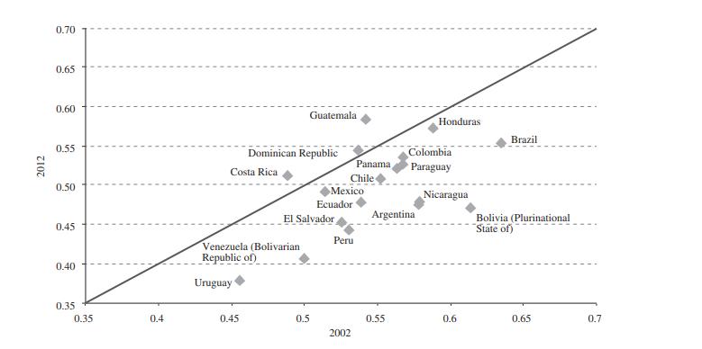
Source: (Amarante et al. 2016)
Figure 2 shows the percentage of wealth held by the top quintile of income earners in the Latin American countries. When the top quintile owns a disproportionately high number compared to the lower quintiles, that shows there is a high level of income inequality. While the percentages in this graph are relatively high, the trend shows that the share of wealth held by the top income earners is falling. The dark grey bar represents 2002, and the light grey bar represents 2012. Only one country has seen an increase in wealth held by the top quintile, which is Costa Rica. Every other country, including the OECD
Figure 1: Latin America (18 countries): Gini Coefficient, around 2002 and 2012
174
countries and potential future OECD countries saw the wealth help by the top quintile fall from 2002 to 2012.
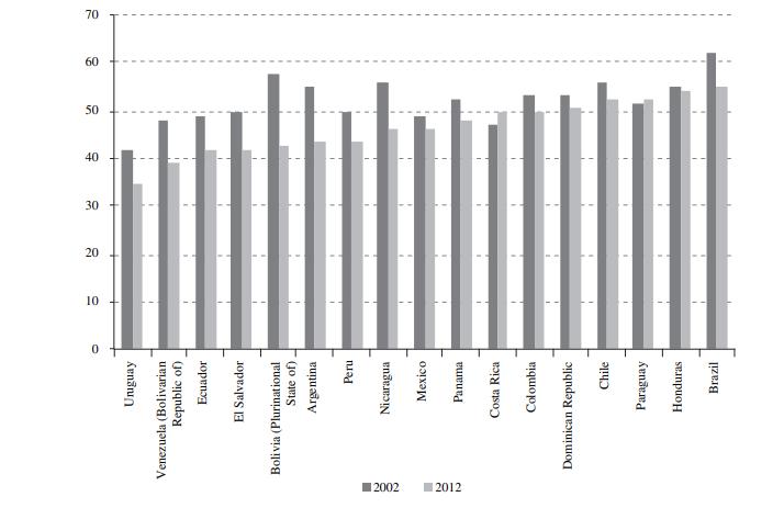
Source: (Amarante at al. 2016)
Figure 3 shows the wealth held by the top 10% in Latin America countries. The difference between this graph and Figure 2 is that this graph has data through 2020. This graph shows that income inequality for the most part is not getting better, and in many cases, is getting worse. Chile, Mexico, and Brazil (OECD countries and candidates) are the top three most unequal countries with the top 10% earners holding around 60%, 58%, and 57% respectively.
Figure 2: Latin America (17 countries): Total Income Share of the Richest Quintile around 2002 and 2012
175
Figure 3: Income Inequality in Latin America: Top 10% Share
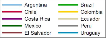
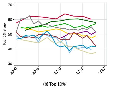
Source: (Rosa et al. 2020)
3.0 LITERATURE REVIEW
Over the past several decades, many European countries went through a massive economic transition from state-owned corporations and agriculture to a more privatized service-based economy (Bucevska 2019). The result of this was an inconsistent, more volatile trend in economic growth and an increase in income inequality. (Bucevska 2019) attempts to find the main factors driving income inequality in three target European countries as this has become a huge global topic. These findings will hopefully provide a road map towards decreasing income equality now and in the future. (Bucevska 2019) finds that the main drivers of income inequality in the selected European countries are the unemployment rate, levels of economic development, and the investment rates. Looking at more demographic factors that have a huge effect are population growth and education. Surprisingly, the results found that the inflation rate and terms of trade were not statistically significant in the selected countries.
176
An empirical model that has been used in global trade theory for many decades is gravity trade and non-gravity trade. Gravity trade is when two countries with similar economic mass (size) trade with each other, and non-gravity trade is the opposite where two countries with different economic mass (size) trades with each other. (Brueckner et al. 2020) study the relationship of non-gravity, bilateral trade between the U.S. and 154 countries, and their levels of income inequality. The main variable chosen in this study besides trade is education. The findings show that when a country has a small percentage of their population educated, an increase in non-gravity trade significantly increases income inequality. Following this, as the population increases education, the correlation between non-gravity trade and income inequality decreases. Countries who are global leaders in education do not have a statistically significant relationship between nongravity trade and income inequality.
Tons of literature look at economic growth, mainly GDP, as an indicator towards income inequality. GDP, however, fails to consider the human elements of income inequality such as human well-being and happiness. (Singha and Singh 2020) argue that is time to start recognizing other models besides growth indicators, like GDP as the metrics used to measure income inequality. Results have shown that overall personal health, labor productivity, and general happiness are greater in poor countries with a more equal distribution of wealth than in wealthier counties with a larger distribution of wealth. While GDP is great for showing the final goods and services sold, taking into consideration sociological, philosophical, and psychological factors can produce much higher growth rates and production output in an economy.
While there is a lot of literature focusing on income inequality and the factors that effect it, very few take the aim of trying to predict the graphical the results. (Checchi 2001) set out to do just that, because she feels that from a policy point of view, it is extremely important to know if a policy change will have a low, moderate, or high change in income inequality. (Checchi 2001) looks at how changes in educational attainment effects income inequality. She finds that the relationship between years spent in school and income inequality is negative, and that it graphically makes a U-shape, with a lower turning point of 6.5 years. It is really important to know that educational
177
attainment is not 1:1 positively linear to consider when making policy changes. Also, (Checchi 2001) finds that income inequality is positively correlated to the capital output ratio and government spending on education, and negatively correlated to per capita income.
(Li and Zou 2002) use a cross-country data set to study how inflation effects income inequality and economic growth in what they consider to be less studied countries (Latin American countries, Asian countries, African countries, etc.). Their results show that inflation worsens income inequality and disproportionately increases the share of wealth for the rich. Surprisingly, they found that while inflation negatively effects the poor and middle class, the results shown were statistically insignificant. Their last result shows that inflation negatively effects economic growth.
Another name for trade percentage of GDP which is used in this paper, is trade openness. (Dorn et al. 2021) study how trade openness affects income inequality in 139 countries from 1970-2014. They use an instrumental variable based on a gravity equation and using a time-varying interaction of geography and impactful natural disasters. The findings are fairly consistent with other research that shows global trade disproportionally helps developing countries and hurts developed countries. In other words, global trade decreases income inequality for developing countries and increases income inequality for developed countries. (Dorn et al. 2021) Note that not every developing country was helped by trade, but overall, the trend is that developing countries are helped more. The developed countries trend of increasing income inequality is a trend of outliers. The type of company that was helped the most (reducing income inequality) were transitioning countries, such as China.
4.0 DATA AND EMPIRICAL METHODOLOGY
4.1 Data
The study uses annual panel data from 2006 to 2020. Data was obtained solely from the World Bank’s World Development Indicators (WDI). Summary statistics for the data are provided in Table 1. (Organization for Economic Co-Operation and Development 2022)
178
Table 1 Summary Statistics
4.2 Empirical Model
Following (Bucevska 2019), this study adapted and modified their model by using mostly similar variables and taking out some variables that did not fit with this study. This study similarly uses the Gini index, GDP, inflation, and unemployment. This study drops grratecaptal, debt, and population. Making slight changes, this study replaces terms of trade (TOT), with trade percent, and education with labor force with basic education. The models in this study could be written as follow:
Variable Observation Mean Std. Dev. Min Max GINI INDEX 79 48.279 4.341 40.9 55.6 INFLATION 105 8.285 9.604 -.0534 50.921 GDP 105 7.98e+10 6.59e+11 2.27e+10 2.62e+12 UNEMPLOYMENT% 105 7.345 2.909 3.21 17.41 TRADE% 105 2.027 18.063 22.105 89.814 LABOR EDUCATION 97 1.029 9.100 40.84 77.36
OLS: Gini Index = β0 + β1 Inflation + β2 GDP + β3 Unemployment% + β4 Trade% + β5 LaborEducation + ε ε = Distance
179
from predicted value and actual value not explained by model
Fixed Effect:
Gini Index = β0 + β1 Inflation + β2 GDP + β3
LaborEducation α + μ
α = Unobserved effects that are invariant
Unemployment% + β4 Trade% + β5
μ = Distance from predicted value and actual value not explained by model
Random Effect:
Gini Index = β0 + β1 Inflation + β2 GDP + β3 Unemployment% + β4 Trade% + β5
LaborEducation + U + W
U = Country specific deviation
W = Year specific deviation
This study compares the results of three different regression models because the results from each one can be interpreted differently. The basic OLS regression compares the relationship between the dependent variable and the independent variables, while looking at the distance from the predicated values and the actual values that are not explained by the model. The Random Effect model looks at the specific deviations in the countries and year. The Fixed Effect model takes into account the unobserved effects that are invariant in the model, while also looking at the distance from predicated values and the actual values that are not explained by the model.
The Gini Index, also known as the Gini Coefficient or Gini Ratio, is the most well know and common indicator for determining income inequality. It Is calculated from the Lorenz Curve which is a graph that essentially shows the distribution of income from a specific population, with a line of perfect equality and the Lorenz Curve which is below the line of perfect equality. The Gini Index is a ratio between these two lines (Bucevska 2019). The Gini Index definition is commonly shared and accepted, and this paper uses the same consistent definition. Many papers examine the relationship between the Gini
180
Index and macroeconomic variables as income inequality is so prevalent around the world. Examples of this can be found in the Literature Review section above.
Independent variables consist of five variables obtained from (The World Bank Group 2022) Appendix A provides data source, acronyms, descriptions, and expected signs. First, Inflation represents the relative change in prices on goods and serves from each country as a percent each year. Second, GDP represents the amount of economic activity taking place in each country. A higher GDP means the country is producing and selling more goods and services, and a low GDP means the country is producing and selling less goods and services. Third, unemployment percent is the percentage of the active labor force that is unemployed. Fourth, trade percent is the percentage of GDP that comes from trade. This is calculated by adding the sum of exports and imports for a specified time period and then dividing it by the same time periods GDP. Fifth, Labor Education is the percentage of the labor force with a basic education, which is defined as completed primary education or lower secondary education. All data, variables, and definitions come from (The World Bank Group 2022).
5.0 EMPIRICAL RESULTS
The empirical estimation results are presented in Table 2. The empirical estimation shows that every variable chosen in this model has a positive correlation to income inequality, except for inflation which is negative. The estimated signs for each variable were predicted as follows: Inflation (+); Trade Percent (+); Unemployment (+); GDP (+); Labor Education (-). The estimated correlations and actual correlations were correct for Trade Percent, Unemployment, GDP, and were incorrect for Inflation and Labor Education.
It should be noted that there were blank data points for the Gini Index and Labor Education for some countries. This was likely due to the difficulty and inconsistency with collecting and reporting this type of data. Due to these blanks, mathematical estimations were applied to the Gini Index variable and the Labor Education variable so the data could be complete and more accurate.
181
Note: *** , **, and * denotes significance at the 1%, 5%, and 10% respectively. Standard errors in parentheses
There are many interpretations that can be made from these results. First, inflation was only significant in the OLS model at 1%, and it is negative which shows that a rise in inflation decreases income inequality. This was surprising because it was assumed that inflation would increase the assets held by the wealthy, and lower the purchasing power of everyone, therefore, increasing income inequality. Second, trade percentage was statistically significant for the fixed effect model at 5%, the random effect model at 10%, and the OLS model at 10%. Trade percentage was assumed to be positive because
Table 2: Regression results for the OECD Latin American Countries
III (OLS) II (Random) I (Fixed) CONSTANT 27.947*** (3.880) 37.521*** (3.696) 38.846*** (3.400) INFLATION -0.119*** (0.032) -0.028 (0.296) 0.01573 (0.027) TRADE% 0.037* (0.020) 0.041* 0.022 0.050** (0.022) UNEMPLOYMENT% 0.917*** (0.112) 0.309*** (0.102) 0.237** (0.095) GDP 3.06e-12*** (4.16e-13) -6.88e-13 (7.35e13) -2.31e-12** (7.81e-13) LABOR EDUCATION 0.178*** (0.038) 0.116*** (0.044) 0.110** (0.042) R2 0.6624 0.1733 0.2183 Number of obs. 105 105 105
Gini Index
182
theoretically it should disproportionately increase the wealth of those who own the trade production. Third, unemployment was statistically significant for the fixed effect model at 5%, the random effect model at 1%, and the OLS model at 1%. It was assumed that unemployment would have a positive correlation because income for the individual decreases drastically (usually to $0), when they are unemployed, however, those who keep their jobs still earn an income, increasing income inequality. Fourth, GDP was statistically significant for the fixed effect model at 5%, and the OLS model at 1%. It was assumed that an increase in GDP would increase income inequality because those that control the means of production would likely become disproportionately wealthier than the average worker. Nationwide production increase correlates to an increase in GDP. Fifth, labor education was statistically significant for the fixed effect model at 1%, the random effect model at 1%, and the OLS model at 1%. It was assumed that as the general population became more educated, the overall wage rate would increase to match the rising skill level, leading to higher wages. The results show that when the education level for those in the work force rise, income inequality rises too. This might occur because the education gap and skill gap increases since not everyone becomes more educated.
Comparing these results to (Bucevska 2019) which is where this study based its model from, the results are fairly consistent. Both studies conclude a negative sign for inflation, a positive sign for unemployment percent, and a positive sign for GDP. While the fixed effect model in this study for GDP has a negative sign, the basic OLS model is more statistically significant with a positive sign. This is consistent with (Rosa et al. 2020) whose OLS model for GDP also has a positive sign. Similarly, (Dorn et al. 2021) shows a positive sign for trade percentage which is consistent with this papers results. While our definitions for education are slightly different, it is still interesting to see that (Bucevska 2019) resulted in a negative sign, while this study consistently resulted in a positive sign for each model. (Li and Zou 2002) also found a negative relationship between primary education and income inequality, as well as a negative sign for inflation which is consistent across all three studies.
It should be noted that the data for this experiment was imperfect which lead to certain variables for the fixed effect model and the random effect model to be statistically
183
insignificant. This data was likely imperfect because of the independent variables chosen might not be good indicators to predict income inequality, as well as the blank data points which were estimated. This can also be shown from the low r-squared fixed effect model and random effect model at .2183 and .1733 respectively. Following this study, different variables should be selected so there is a higher correlation between the dependent and independent variables. The amount of years that this study examines should be longer, preferably 20 years minimum.
6.0 CONCLUSION
In summary, there are many different variables that impact income inequality in the OECD Latin American Countries. Knowing the variables that increase or decrease income inequality is extremely important since this has been a growing concern globally. The results show that trade percentage, unemployment percentage, and labor education result in higher income inequality, while inflation and GDP result in lower income inequality. Given that this study uses an odd number of variables, more macroeconomic variables increase income inequality than decreases income inequality. However, if more variables were used, this conclusion may differ.
While income inequality is not a good thing, it can certainly be argued that trade percentage and labor education are generally positive for an economy / society. Trade allows a country to make money on their surplus production and provide the population with products and services that could not be efficiently produced in their borders. A more educated labor force translates to an increase in production, as well as innovation. Therefore, before changing or creating any new policies, every potential outcome must be thought of and analyzed. On the other side, it makes sense that unemployment increases income inequality because not everyone becomes unemployed, so those who keep their jobs earn a significantly higher income than those who lost their jobs. Unemployment percentage also had the highest effect on income inequality at 0.917, so based on these results, it is logical that the first policy recommendation should be towards decreasing unemployment / maximize employment.
184
Having an understanding about which variables effect income inequality is necessary for effective policy change. The hope of this study is to further examine other variables that have an impact on income inequality and compare and contrast the results to the vast amount of literature on this topic. While this study solely focuses on OECD countries in Latin America, the results can be used for policy changes all around the world. Comparing the results to other studies that looked at different countries, both developed and developing, who also used different time frames, and seeing similar results shows that the effects of these variables apply globally. Ideally, this study will add a new perspective to the other literature that will expand and enhance the current knowledge around global income inequality. With enough knowledge on which variables have the biggest impact around the world, effective policy can be made / changed to reduce the gap on income inequality in every country, regardless of size.
If this study were to be redone, many changes would have to be made. First, the models would need to have many more independent variables than just five. There are so many possible variables that effect income inequality that five is not enough. Also, further investigation will be needed to figure out why inflation was not statistically significant for the fixed effect model or the random effect model. Second, the study should use a longer time-frame than just 15 years. The issue of rising income inequality dates back further than 15 years, so a longer time frame would be needed. Third, it would be helpful to compare these results to other Latin American countries that have no relationship to the OECD to see what effects the OECD has on income inequality. At its core, this study is very basic with lots of room for improvement in later versions.
Appendix
185
A: Variable Description and Data Source
Gini Index
Represents income inequality. The gap between the Lorenz Curve and the line of perfect equality
Inflation The rate in which prices rise and purchasing power declines
World Development Indicators
World Development Indicators
GDP The final market value of products and services produced within a country's borders
World Development Indicators
Unemployment % The percentage of the active labor force currently unemployed
World Development Indicators
Trade % The sum of exports and imports of goods and services divided by GDP
World Development Indicators
Labor Education
The percentage of the active labor force with basic education (primary or lower secondary)
-
Acronym Description Data source Expected Sign
+
+
+
+
+
World Development Indicators 186
Bibliography
Amarante, Verónica, Marco Galván, and Xavier Mancero. 2016. "Inequality in Latin America: a global measurement." Cepal Review 26-44.
Brueckner, Markus, Ngo Van Long, and Joaquin Vespignani. 2020. "Trade, Education, and Income Inequality." CESifo (Munich Society for the Promotion of Economic Research).
Bucevska, Vesna. 2019. "Determinants of Income Inequality in EU Candidate Countries: A Panel Analysis." Economic Themes (Economic Themes) 57 (4): 397-413.
Checchi, Daniele. 2001. "Education, Inequality and Income Inequality ." Distributional Analysis Research Programme .
Dorn, Florian, Clemens Fuest, and Niklas Potrafke. 2021. "Trade Openness and Income Inequality: New Empirical Evidence." ifo Institut .
Li, Hongyi, and Heng-fu Zou. 2002. "Inflation, Growth, and Income Distribution: A Cross-Country Study." ANNALS OF ECONOMICS AND FINANCE 85–101.
Organization for Economic Co-Operation and Development. 2022. About Us: Organization for Economic Co-Operation and Development. Accessed April 7, 2022. https://www.oecd.org/about/.
Rosa, Mauricio De, Ignacio Flores, and Marc Morgan. 2020. Inequality in Latin America Revisited: Insights from Distributional National Accounts. Issue Brief , World Inequality Lab.
Singha, Shashank Vikram Pratap, and Sumanjeet Singh. 2020. "Exploring the Linkage between Income Inequality, GDP and Human Well-Being." Business and Economic Research 621-634.
The World Bank Group. 2022. World Development Indicators. April 8. Accessed April 9, 2022. https://databank.worldbank.org/source/world-development-indicators.
187
Causal Relationship Between Defense Spending and Economic Growth in Countries with Different Income Levels
Kyle Sampson
Abstract:
This paper addresses the relationship between defense spending and economic growth for various economies with different income levels. Using time series annual data, the Granger causality test was conducted. This study looks to determine whether the direction of causality in these economies is different in low−income, middle income, and high−income countries.
JEL Classification: O10, H56
Keywords: Economic Development, National Security
a Department of Economics, Bryant University, 1150 Douglas Pike, Smithfield, RI02917. Phone: (401) 232-6379. Email: ksampson1@bryant.edu.
188
There have been various discussions as to the possible causal relationship between defense spending and economic growth. Other studies have been conducted to research things related to this relationship but none of them discuss this direct relationship.
This study aims to enhance understanding of the relationship between defense spending and economic growth for countries at the three different income levels (Lower, Middle, Upper). From a policy perspective, this analysis is important because it will provide an argument for legislation to be passed or denied regarding defense spending to spring economic growth. The relevance of this study is that countries are always looking to increase the growth of their economy and there could be a direct relationship between this and defense spending. This study goes further to examine this relationship possibility for countries with different income levels in order to see if there is a relationship as some levels but not others.
In order to investigate the relationship between defense spending and economic growth, this study looks to see if the causality is from defense spending to economic growth or vice versa. The Granger causality test is used to compare the no causality or unidirectional/bi-directional relationship between defense spending and economic growth.
The rest of the paper is organized as follows: Section 2 gives a brief literature review. Section 3 outlines the empirical model. Data and estimation methodology are discussed in section 4. Finally, section 5 presents and discusses the empirical results. This is followed by a conclusion in section 6.
1.0
INTRODUCTION
189
2.0 TREND OF MILITARY EXPENDITURE AND GDP
When starting to investigate the general topic of defense spending, the first thing to look at is the overall amount of money put into it by the world. My initial expectation was to see rising times and falling times depending on the overall tension and potential for conflicts to break out around the world. Looking at Figure 1 below, you can see that from 1980 to 2010 there is a constant increase in dollars spent with extreme growth shown from 2000 to 2010. Around 2012 there is a plateau followed by the only decrease coming from 2014 to 2015. In recent years the increase has started back up and currently shows no signs of slowing down. It seems as though the world is in a never-ending arms race to gain military superiority.
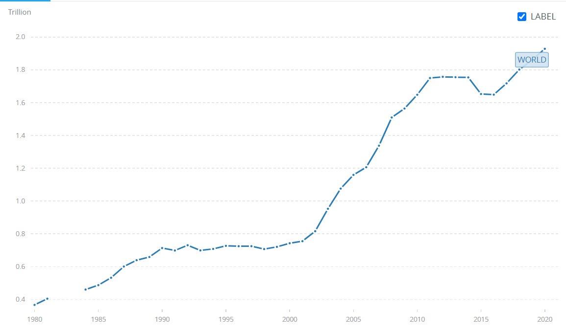 Figure 1: Military Expenditure (current USD)
190
(Source: The World Bank)
Rather than just look at the USD spent over time; Figure 2 shows the military expenditure as a percentage of GDP. This gives a better overall view of how much of the world’s money is going into Military spending. This shows that even though the USD has increased over time, the actual percent of GDP has lowered over time. In the last year of the chart, 2019 to 2020 showed an uptick in the percent of GDP going into Military spending. This can possibly be explained by keeping military spending stagnant even though overall GDP dropped slightly from 2019 to 2020. This presumed drop in overall GDP would be explained by the outbreak of the Covid-19 virus.
2: Military Expenditure (% of GDP)
(Source: The World Bank)
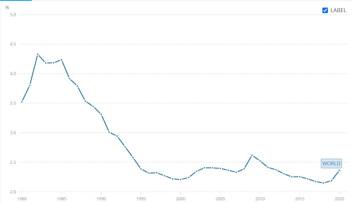 Figure
191
Looking into the annual percentage of GDP growth in figure 3, you can see that there is a drastic drop from 2019 to 2020. This can be explained by the Covid19 outbreak and shutdowns of many major cities across the world.
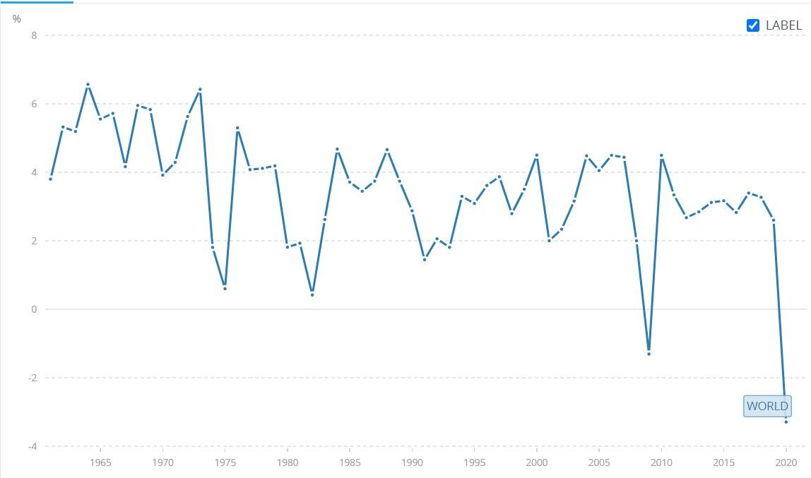
(Source: The World Bank)
3.0 LITERATURE REVIEW
Tiwari, (2011) investigates the relationship of defense spending and economic growth on a smaller scale, looking at India specifically. They confirmed a long-term relationship between the variables which indicated a positive effect of defense spending on economic growth. After running a Granger causality test, they identified a bidirectional causal relationship between defense spending and economic growth.
Figure 3: GDP Growth (Annual %)
192
Dunne, (2011) uses an augmented Solow-Swan model and estimates both with panel and time series methods in order to give evidence to support the effects of defense spending in the EU15. Unlike the findings of (Tiwari, 2011), the data suggested that this defense spending did not promote economic growth in the region.
Kunu, (2016) uses various developing countries, specifically the Middle East, to look at the relationship between defense spending and economic growth. The question that is researched is whether increased defense spending has a negative impact on the economic growth of these countries. Being poorer countries that are constantly militarized, a lot of their overall spending goes to defense spending which could stunt economic growth as there may not be enough funding left for more important areas.
Shahbaz, (2012) investigates this relationship between defense spending and economic growth much like (Tiwari, 2011), only it looks at Portugal rather than India. Different than previous papers, they discovered a U-shaped correlation between defense spending and economic growth. Rather than a bi-directional relationship, they found a uni-directional relationship from defense spending to economic growth. It was determined that Portugal could stimulate economic growth by increasing their defense spending.
Mohanty, (2020) follows (Tiwari, 2011) very closely. He also investigates the relationship of defense spending and economic growth in India but compares older data to newer data on the subject rather than just using one and going with it. It was found that
193
capital defense expenditure has a significant impact on economic growth while revenue defense expenditure has no significant impact. This study adds additional evidence to support that defense spending should be encouraged in order to stimulate economic growth in India specifically. Frederiksen, (1991) researches the Philippines, specifically the relationship between defense spending and economic growth. This paper looks deeper into the implications that this research has on Phillippine policy development.
4.0 DATA AND EMPIRICAL METHODOLOGY 4.1 Data
The study uses panel data from 1989 to 2020. Data were obtained from the Bureau of Economic Analysis (BEA) website World Development Indicators. Publicly available BEA data excludes countries where less than $500,000 is invested and avoids disclosure of individual firm data. The variables used in this study and the definitions are LogGDP (log of Gross Domestic Product) and LogMIL (log of Military Expenditure).
GDP can be defined as the total value of all finished goods produced within a country in a given time period. Military Expenditure can be defined as the number of financial resources designated to raising or maintaining the military of a country.
The aim of this study is to determine the causality between both variables in each country. The data used are in terms of United States Dollars (USD). The countries used in each income level were selected based on location and data availability. The number of
194
countries selected at each level is constricted due to lack of data available for certain countries.
4.2 Empirical Model
Granger was well known for his granger causality test. This test ran two variables to test for a causal relationship between them. It ended up with one of four possible outcomes; No causality between GDP and MIL, GDP causes MIL, MIL causes GDP, or there is a bi-directional causality meaning that GDP causes MIL and MIL causes GDP simultaneously.
There are five steps that must be followed in order to properly run the granger causality test and they are as follows:
1) Test for the presence of a unit root using the Augmented Dickey-Fuller Test (ADF).
2) Take the first difference of the in the presence of unit root and conduct the ADF test on the differenced data.
3) Exclude countries where one of the variables is non-stationary and the other is stationary
4) Estimate for co-integration using the same order of integrated variables.
5) Based on these results, use the VAR or VEC test for causality.
Model:
The first test ran is to determine if the data is non-stationary, so we check to see if they have unit roots. To test for a unit root we use the ADF test using the equations below.
195
ADF test for unit route:
Given the results of the ADF test, the next step is to test for co-integration. Each of the variables must be tested for each country, the Johansen method is used to do this.
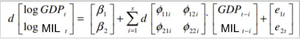
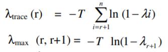
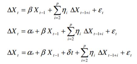
Test for co-integration:
The results of the co-integration test can be seen in table 2. If the variables are not co-integrated, the VAR test is used to test for granger causality. For the countries where the two variables are co-integrated, the VEC test is used to test for causality.
VAR test for the countries that were not co-integrated:
Using the correct lag length is very important to make sure that the results are not misspecified while still not wasting the degrees of freedom.
SBC test used to determine correct lag length:
VEC model by Granger:
196
5.0 EMPIRICAL RESULTS
In the introduction of this study, it is stated that the purpose of this study is to test the direction of causality between defense spending and economic growth. The results of the ADF test indicates that LogGDP and LogMIL both have unit roots in the level data. When there are unit roots, the data must be differentiated for the series to be stationary. Misspecification occurs if the data is not differentiated. The added in factor of this study is that the data is split to look into the different income levels of the countries.
Table two shows the countries in which the co-integration test was used, and the variables were not mis specified. 14 of the countries data were not mis specified which resulted in valid responses for the granger causality test.
As seen in table 3, the results of the Granger test for Low-Income Countries were valid for two countries, (Mozambique and Ethiopia). Mozambique showed bi-directional causality while Ethiopia showed no causality. These two very different results cause there to be no distinct trend in the Low-Income Countries.
For Middle Income Countries, five had valid Granger results. Three of these countries had no causality, while Bolivia has uni-directional causality from economic growth rate to defense spending. Ecuador showed bi-directional causality, Middle Income Countries also showed no distinct trend in results.
High Income Countries had more data available, with seven countries having valid Granger results. Sweden showed bi-directional causality, while three countries showed uni-directional causality and three showed no causality. This split shows no distinct trend for High Income Countries.
197
The main purpose of this paper was to investigate the relationship between defense spending and economic growth in countries of different incomes. Overall, three countries showed a bi-directional relationship. Four countries showed a uni-directional causal relationship from economic growth to defense spending. No countries showed a uni-directional causal relationship from defense spending to economic growth. Seven countries showed no causal relationship between defense spending and economic growth. Based on the results, this study favors the hypothesis that there is no distinct causal relationship between economic growth and defense spending in countries of different income levels. There are split results in each of the income brackets, show no distinct trend
In the future, I would like to research the legislation that is in place in the countries with different uni-directional or bi-directional causal relationships shown. Is there legislation that forces these relationships and if so, could other countries put similar laws in place to facilitate this relationship?
5.0 CONCLUSION
198
APPENDIX
Table 1: ADF Test
Note: *** , **, and * denotes significance at the 1%, 5%, and 10% respectively.
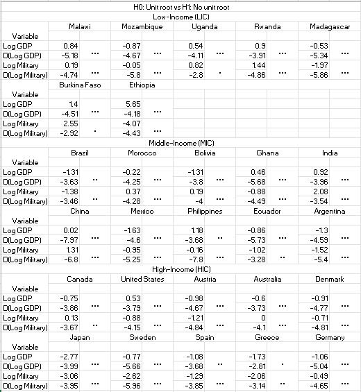
199
Table 2: Co-Integration Test
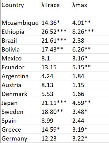
200
Table 3: Granger Test
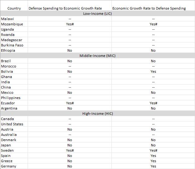
201
BIBLIOGRAPHY
Dunne, J. P. (2011). Defence Spending and Economic Growth in the EU15. 16.
Frederiksen, P. C. (1991). Economic Growth and Defense Spending: Evidence on Causality for Selected Asian Countries. Journal of Philippine Development, 17.
Kunu, S. (2016). Conflict, Defense Spending and Economic Growth in the Middle-East: A Panel Data Analysis. International Journal of Economics and Financial Issues, 8.
Mohanty, R. K. (2020). Does Defence Spending and its Composition Affect Economic Growth in India? The Journal of Applied Economic Research 14, 24.
Ranis, G. (2004). Human Development and Economic Growth. 15.
Shahbaz, M. (2012). Should Portuguese Economy Invest in Defense Spending? A Revisit. Munich Person RePEc Archive, 30.
Tiwari, A. (2011). Does Defence Spending Stimulate Economic Growth in India? Munich Personal RePEc Archive, 44.
202
International Integration and Export-Led Growth in Latin America: A Panel Data Analysis
James Titus
Abstract:
This paper investigates the potential determinants for international integration and effects of export-led growth in Latin American countries to determine the most effective measure of growth in the countries. The study incorporates information asymmetry into a GDP per capita growth model to examine the influence of openness, human capital, export diversity, and more. While examining data from World Bank development indicators, it has been shown that there are at least nine different variables that provide relevant data to create a functional model. The results show that there are many applicable determinants that can be used in the model without over-correlation. Using a model from a previous study in Asian countries, the determinants are expected to be able to be used in the same manner for these Latin American and Caribbean countries. By analyzing the top 10 countries by GDP, the model will investigate the correlation between export-led growth-related variables and economic success in the countries.
JEL Classification: O24, O40
Keywords: Economic Growth, Latin America, Economic Crisis, Determinants, Export-Led Growth, International Integration
Department of Economics, Bryant University, 1150 Douglas Pike, Smithfield, RI, 02917.
Email: jtitus3@bryant.edu.
203
1.0 INTRODUCTION
International integration is a newer means for understanding GDP per capita growth. It is very useful in creating a “global” view of a country’s growth, and in this situation, the growth of Latin American countries over the last 20 years. As the world becomes bigger, the connections have become much smaller and allowed for more international trade and work than ever before. While examining the work of Ramanayake and Lee (2015) for Asian countries, the same principles can be applied to these Latin American and Caribbean countries.
To successfully determine the most relevant inputs for the recent GDP per capita growth in this region, there must be a diagnosis of 1. what factors directly contribute to international integration in the country, and 2. what among those determinants holds the most impact.
The research was guided by the need to understand globalization and its positive effects on economic growth in these rapidly developing countries. While previously, determinants such as domestic investment and manufacturing could explain GDP per capita growth, the world has evolved much more into an interconnected, global economy. The need for an “international integration” type of determinant is important for understanding the true impact and importance of factors such as openness, export-led growth, and foreign direct investment on overall growth in these economies. Export-led growth will provide the most expansive view of GDP per capita growth due to its depth and the large pool of data.
The rest of the paper is organized as follows: Section 2 gives a brief literature review. Section 3 outlines the empirical model. Data and estimation methodology are discussed in section 4. Finally, section 5 presents and discusses the empirical results. This is followed by a conclusion in section 6.
2.0 TREND
Figure 1 shows the relationship between export growth percentage and GDP per capita growth. In this scatter plot, it is shown that there is a slight positive correlation between higher export growth and GDP per capita growth rate for these countries. This is shown on the next page.
204
Source: World Bank Database UNCTAD
Figure 2 shows a similar story when considering GDP per capita growth rate compared to population growth. A higher level of population growth contributes to a lower overall GDP per capita due to the higher amount of people in the country. Here, we can see a slight negative correlation between GDP per capita growth rate and this variable.
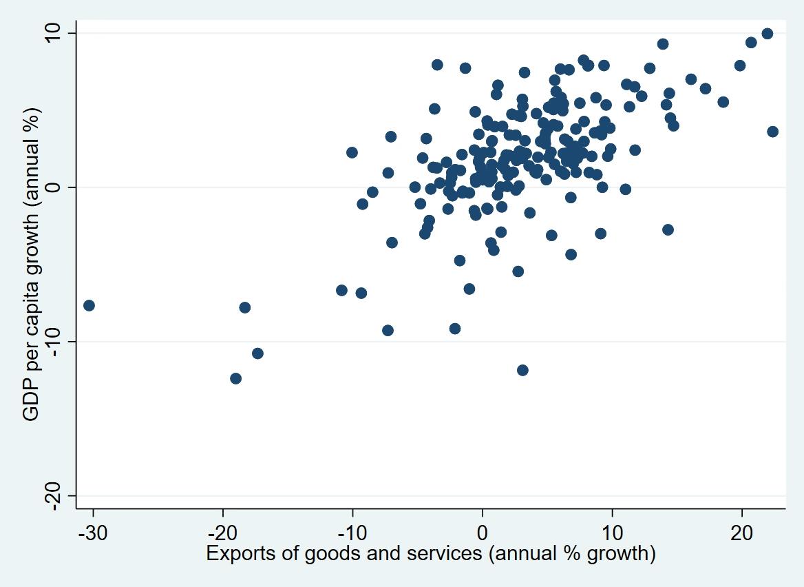 Figure 1: GDP per capita growth rate (annual %) vs. Exports of goods and services (annual % growth)
205
3.0 LITERATURE REVIEW
While the focus of the initial paper by Ramanayake and Lee (2015) was economic growth determinants, the focus was mostly on the international integration determinants, such as export growth and foreign direct investment. Foreign direct investment has been a popularly used determinant for economic growth research (Accolley, 2003; Majidi et al., 2017; Greaney and Kiyota, 2020). However, export growth is a more complicated topic that could potentially create a more interesting response.
According to Bahramian and Saliminezhad (2020), based on the theories of trade and growth, connection flows from export growth to economic development as export-led growth constitutes a part of the aggregate output. Simply put, export-led growth should provide a very direct correlation for economic growth and development.
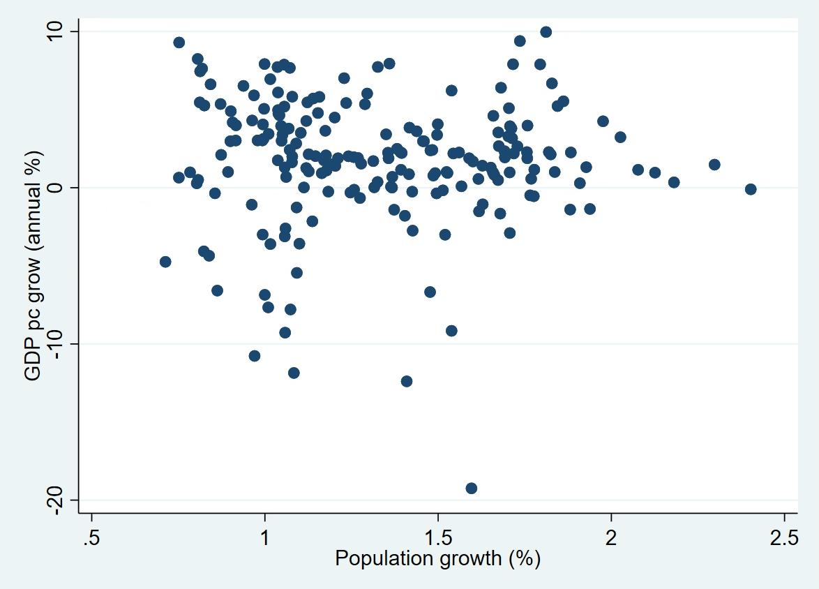 Figure 2: GDP per capita growth (annual %) vs. Population growth (%)
Source: World Bank Database UNCTAD
Figure 2: GDP per capita growth (annual %) vs. Population growth (%)
Source: World Bank Database UNCTAD
206
Hagemejer and Mućk (2018) examined the determinants for export growth in Central European countries, which provide applicable information for the Latin American and Caribbean countries examined in this report. Through direct (increase in demand and subsequent increase in the physical output) and indirect (through the effects of specialization and related productivity boosts) measures, the authors found that export expansion allows for increased imports of more advanced intermediates and investment goods that provide additional gains to productivity.
Another article that considered export-led growth comes from Trošt and Bojnec (2016), who consider export-led growth in Slovenia and Estonia. These countries are useful for comparing growth effects in Latin American countries due to their open and export-oriented economies, which these high-GDP Latin American and Caribbean countries are comparable. Some important institutional decisions to consider are that the Slovenian government provides support for the internationalization of enterprises, which has become one of the most important strategies for firms to achieve sustainable growth. In addition, the Estonian economic policy main principles are flexibility and trade openness. It is also considered an e-business country with a favorable business climate and cost advantages opened to growth. Both countries have forward-thinking leadership that allows for export-led growth to prosper.
When looking at international integration, there is more than simply export growth to consider. Arespa (2014) provides a look at international integration and specifically financial integration on economic volatility, which is especially relevant for GDP per capita growth. The author writes that financial integration is supposed to serve as a cushion against adverse domestic shocks by allowing for lending and borrowing from abroad, which should lead to a decline in consumption volatility. However, this integration also increases the potential for the magnification of financial shocks, so output and investment volatility may increase as well. Knowing this information, it will be interesting to discover what the case may be in Latin American countries.
Yildirim and Gökalp (2015) gave insight into what factors could potentially halt economic growth in Latin American countries. According to the literature, it is the arrangements of political institutions, which are generally inconsistent with the interests of citizens. This includes providing bad public services, manipulation in the judicial system, corruption, bribery, tax evasion, ill-defined property rights, and the existence of inefficient institutions. This
207
information is important to note because it can explain the reasoning behind a lack of GDP per capita growth, as well as an inefficiency in international integration. While many Latin American countries are globalizing, poor institutional effectiveness could play a large role in stunting economic growth.
4.0 DATA AND EMPIRICAL METHODOLOGY
4.1 Data
The study uses annual panel data from 2001 to 2020. Data were obtained from the Bureau of Economic Analysis (BEA) website World Development Indicators. WDI data for multiple variables were taken from the top 10 Latin American and Caribbean countries by GDP, which are as follows: Brazil, Mexico, Argentina, Colombia, Chile, Peru, Ecuador, Dominican Republic, Guatemala, and Panama. Summary statistics for the data are provided in Table 1, which continues onto the next page.
Table 1: Summary Statistics
Variable Observation Mean St. Dev Min Max Y (GDP per capita growth) 200 1.730118 4.101681 -19.24428 9.973723 LN_INTGDP 200 8.871222 .4297838 8.0685 9.620661 POPGROW 200 1.331944 .3523861 .7128728 2.402401 PCAP 200 22.48733 6.105473 10.85391 44.3086 HCAP 161 94.05257 3.946097 81.78003 99.49576 FDI 200 3.57684 2.743199 -5.088204 16.22949 EXGROW 199 3.096786 6.903832 -30.31869 22.36241 OPEN 200 56.73508 28.01594 21.85225 166.6982 FOODDIVERS 197 29.58366 19.22373 2.874969 85.14786 COMDIVERS 200 24.06448 18.60071 -9.35039 66.15672 LIFEXP 190 74.74373 2.395634 68.304 80.181 DEMOC 200 49.27926 16.54461 15.60976 87.37864 208
4.2 Empirical Model
Following Ramanayake and Lee (2015), this study adapted and modified the original GDP per capita growth rate model to incorporate different proxies for openness, democracy, and export diversification. The new model has some changes, which are as follows:
Yit = β1LN_INTGDPit + β2POPGROWTHit + β3HCAPit + β4PCAPit + β5FDIit + β6EXGROWit + β7OPENit + β8FOODDIVERSit + β9COMDIVERSit + β10LIFEXPit + β11DEMOCit + Eit
Yit is the GDP per capita growth rate of country i at year t. Yit is used as an endogenous variable.
LN_INTGDPit is the log of initial GDP per capita of a country i expressed in constant US dollars. POPGROWTHit is the population growth. HCAPit is human capital, measured as primary school enrollment. PCAPit is gross capital formation as a percentage of GDP. FDIit is foreign direct investment as a percentage of GDP. The variables for international integration include EXGROWit (growth in exports as a percentage of GDP), OPENit (trade as a percentage of GDP), FOODDIVERSit (percentage of exports related to food and drink), and COMDIVERSit (percentage of exports related to computers and communication). The other controls include LIFEXPit as life expectancy, and DEMOCit as government effectiveness. Eit is the error term.
5.0 EMPIRICAL RESULTS
5.1 Results
The empirical estimation results are shown in Table 2. The results for the ordinary least squares, random effect, and fixed effect regressions are in order and labeled. For the purposes of this research, the fixed effect model was the most relevant in determining the factors that affected GDP per capita growth the most. In this regression, it is seen that the significant variables were POPGROW, PCAP, EXGROW, and LIFEXP, with the first three being significant at the 1% level and LIFEXP being significant at the 5% level. For the random effect regression and the OLS regression, POPGROW, PCAP, and EXGROW were all also significant at the 1% level.
209
Table 2: Regression Results
Note: *** , **, and * denotes significance at the 1%, 5%, and 10% respectively. Standard errors in parentheses. 161 observations, 10 groups.R-squared values:
// RE (.4537) // FE (.4928)
5.2 Empirical Analysis
Variables OLS Random Effect Fixed Effect LN_INTGDP -1.157723 (-1.16) -1.157723 (-1.16) 5.181505 (1.39) POPGROW -3.430109 *** (-3.74) -3.430109 *** (-3.74) -4.956565 *** (-3.94) PCAP .2452953 *** (3.86) .2452953 *** (3.86) .354896 *** (3.35) HCAP -0.649267 (-0.86) -0.649267 (-0.86) .0419851 (0.43) FDI .0977021 (0.80) .0977021 (0.80) .0628789 (0.47) EXGROW .252488 *** (6.95) .252488 *** (6.95) .2830525 (7.81) *** OPEN .007815 (0.51) .007815 (0.51) -.0095825 (-0.40) FOODDIVERS .0090212 (0.63) .0090212 (0.63) .0178033 (0.93) COMDIVERS .0086866 (0.49) .0086866 (0.49) .0412739 (1.35) LIFEXP -.071716 (-0.54) -.071716 (-0.54) -1.02085 ** (-.2.29) DEMOC -.0236043 (-1.09) -.0236043 (-1.09) -.0447151 (-1.11) _CONS 22.49514 (2.11) 22.49514 (2.11) 27.29583 (1.57)
OLS (.4432)
210
Population growth, gross capital formation, and export growth were all significant at the 1% level. In the fixed effect regression analysis, life expectancy was significant at the 5% level. Population growth and life expectancy both had a slight negative impact on GDP per capita growth rate, whereas gross capital formation and export growth had a positive impact on GDP per capita growth rate. These findings were consistent with the initial study by Ramanayake and Lee (2015) and Hagemejer and Mućk (2018). Interestingly, both openness and foreign direct investment were not significant in any of the three regressions that were run for this dataset. This is in contrast to the other studies examined, where both of these variables were relatively significant. Foreign direct investment in particular has been consistently linked to economic growth in many different academic studies and literature reviews. Despite this, export growth and gross capital formation have proven to be positively impactful on the per capita GDP growth in Latin America. The empirical results suggest that the more investment in international trade and integration there is, the higher chance that the people within the country will prosper.
5.3 Policy Implications
In terms of policy implications, the data suggests that there needs to be a shift in better quality shipping and exporting infrastructure in these countries to create more robust economies. In addition to the infrastructure, the corruption in these countries needs to be handled. Although corruption can sometimes be a positive for economic growth and consumption, in the case of Latin America, it has led to many more problems than successes. The writings of Yildirim and Gökalp (2015) show true in this analysis, mostly due to ineffective government leaders. While there is plenty of capital investment, there needs to be more institutional investment to create a more hospitable economic environment.
5.3 Limitations
Limitations of the study come down to some gaps in data for certain determinants that needed proxies, as well as Brazil and Mexico being a fair bit more economically intense than the other 8 countries listed. A lack of data for many different determinants, such as secondary school enrollment (human capital) and export diversification, made the search for proxies very difficult. In future studies, the need to purchase more accurate data will be considered. In addition, the model used may have potentially had too much collinearity due to the number of variables used. Some of the variables in the original model overlapped already, so with the addition of more
211
variables and proxies, this may have stretched the data too thin, as well as taken relevancy away from some variables that were predicted to be relevant (FDI and openness, for example). In a report with less of a time constraint, this would not be as much of an issue.
6.0 CONCLUSION
In summary, Latin American countries should be focused on gaining more gross capital formation and export growth to ensure per capita GDP growth within the countries. More intensive research must be done within this economic model as well as modifying the model to provide even clearer results. While the majority of these Latin American countries are making a slight recovery from years prior, particularly with COVID-19 residual effects still looming, most of these countries will be set to make an impact on GDP per capita growth with more investment in their manufacturing and exporting infrastructure.
Despite prior research showing that foreign direct investment and openness were important determining factors for economic growth, it is still perplexing that in Latin America, this was not the case. Further research must be done to tie together the findings of the previous literature and what was found in this study.
Overall, this analysis was successful in showing that international integration does play a role in the per capita GDP growth of Latin American countries. International integration has been considered a very integral part of world development, so it is good to see this opinion be backed up with empirical data. Export growth is proven to be crucial in per capita GDP development in Latin America.
Appendix: Variable Description from World Bank
Yit is the GDP per capita growth rate of country i at year t
212
LN_INTGDPit is the log of initial GDP per capita of a country i expressed in constant US dollars
POPGROWTHit is the population growth
HCAPit is human capital, measured as primary school enrollment
PCAPit is gross capital formation as a percentage of GDP
FDIit is foreign direct investment
EXGROWit is growth in exports by percentage
OPENit is trade % of GDP
FOODDIVERSit is food exports
COMDIVERSit is computer and communication exports
LIFEXPit is life expectancy
DEMOCit is government effectiveness
Eit is the error term Bibliography
213
Accolley, D. (2003). The Determinants and Impacts of Foreign Direct Investment. Munich Personal RePEc Archive, 2-66.
Arespa, M. (2015). Macroeconomic Volatility and International Integration. Bulletin of Economic Research, October 2015, 393-410.
Bahramian and Saliminezhad (2020). On the relationship between Export and Economic Growth: A Nonparametric Causality-in-Quantiles Approach for Turkey. Journal of International Trade and Economic Development, January 2020, 131-145.
Greaney, T., & Kiyota, K. (2020). Japan's Outward FDI Potential. Keio-IES Discussion Paper Series, 3-33.
Hagemejer, J., & Mućk, J. (2018). Export-Led Growth and Its Determinants: Evidence from Central and Eastern European Countries. World Economy, July 2019, 1994-2025.
Majidi, A. F., Hashembeigi, H., Afshar, P. A., & Hashembeigi, V. (2017). Determinant of FDI: Evidence from Organization of the Petroleum Exporting Countries (OPEC). Asian Economic and Financial Review, 258-266.
Ramanayake, S. S., & Lee, K. (2015). Does openness lead to sustained economic growth? Export growth versus other variables as determinants of economic growth. Journal of the Asia Pacific Economy, 1-22.
The World Bank. (2022, April 1). World Bank Development Indicators. Retrieved from worldbank.org: https://databank.worldbank.org/reports.aspx?source=world-developmentindicators#
Trošt, M., & Bojnec, S. (2016). Export-Led Growth: The Case of the Slovenian and Estonian Economies. Post-Communist Economies, September 2016, 373-383.
Yildirim, A., & Gökalp, M. F. (2016). Institutions and Economic Performance: A Review on the Developing Countries. Procedia Economics and Finance, 347-359.
214
Granger Causality of the Relationship Between Tourist Flows and Household Expenditure in Jamaica
Ben Williamsa
Keynesians propose that increases in tourist arrivals are associated with an expansion in private spending through the multiplier effect. To test this hypothesis, this study augments a simple consumption function with tourist arrivals and employs the dynamic OLS method to compute the short and long run relationships of the variables. Time series data from 1980-2019 is used to test if tourist arrivals Granger cause household expenditure. The results show that there is no relationship between tourist arrivals and household expenditure in Jamaica and tourist arrivals do not Granger cause household expenditure.
JEL Classification: J1, C32
Keywords: Tourism.
a Department of Economics, Bryant University, 1150 Douglas Pike, Smithfield, RI 02917.
Phone: (401) 354-9992. Email: bwilliams11@bryant.edu
215
1.0 INTRODUCTION
Keynesians propose that tourist arrivals affect household expenditure through the multiplier effect. Under this theory, private household expenditure should increase as tourist arrivals increase. As outlined by Tse (1998) pp. 233, “Tourism spending represents a net demand for domestic output. Such a net demand provides incomes in the economy…. recipients of this extra income in turn raise their consumption, creating further production and income gains in an endless but rapidly diminishing chain”. From a policy perspective, this is especially important to the country of Jamaica because of its reliance on tourism for its economy. The onset of the pandemic has negatively affected many countries economically, especially those which rely on aggregate demand from tourism. This study hopes to shed light on the relationship between tourist flows and household expenditure to provide policy recommendations in the wake of the pandemic. The relevance of this study is that it will build upon previous literature investigating the relationship between tourist inflows in the Caribbean and the Gulf of Mexico. This paper is guided by three primary research objectives: First it investigates the Granger causality of the relationship between tourist flows and household expenditure in Jamaica leading up to the pandemic; second, it will attempt to explain the reasoning behind the relationship between the two variables; lastly, this paper will provide policy suggestions to improve tourist flows and household expenditure in the wake of the pandemic. This paper serves a purpose based on the outcome of the results: first, it seeks to answer the question, does tourism affect household expenditures in tourism-dependent economies? If it does, how can countries rebuild their tourist sector in the wake of Covid and if it does not, what are some solutions to help these countries rebound from the effects of the pandemic?
2.0 TRENDS
Tourism is a major contributor to global trade. In 2019, global tourism was the thirdlargest export category, making up 7% of global trade (UNWTO, 2020). In addition, 100 to 120 million tourism jobs worldwide were at risk because of the pandemic, leading to a fall in export revenues from tourism between $910 billion and $1.2 trillion (UNWTO, 2020). Preliminary data from the UNWTO states that international arrivals were down 62% in the third and fourth quarter of 2021 from 2019 levels and down 65% in December 2021 from 2019. Even with the
216
swift rollout of vaccinations, international arrivals remain well below pre-pandemic levels, putting Jamaican and other small-island nations in the Caribbean’s economy and employment levels at risk. Figure 1 shows the GDP contraction of Jamaica and comparable nations in 2020 to the largest GDP shock in the period of 1975-2019. For many in the Caribbean, 2020 had the largest negative contribution to GDP in 45 years. This further emphasizes the objective of the paper to determine the relationship between tourist arrivals and household expenditures in Jamaica.
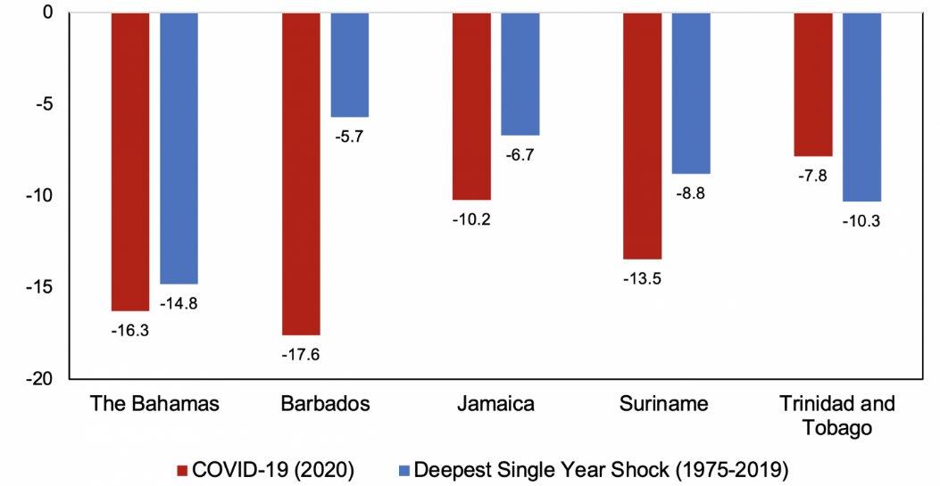
Source: Caribbean Quarterly Bulletin (May 2021)
Figure 2 shows the increase in tourist arrivals from 1980 through 2019 in Jamaica. Form 2000 to 2019, tourist arrivals doubled in Jamaica, showing the growth of the industry in the island nation. There has been a steady increase each year outside of global shocks such as the 2008 financial crisis.
Figure 1: GDP Contraction in 2020 vs Largest Historical Shock from 1975 to 2019 (%)
217
Figure 2: Tourist Arrivals into Jamaica
International tourism, number of arrivals

Source: World Bank World Development Indicators
3.0 LITERATURE REVIEW
Tourist flows from the World Bank Development Indicators indicates the total number of tourist arrivals from international tourism. This separates the statistic from other figures because it includes stopovers under 24 hours such as from cruise liners that port for the day which is important because of the spending that comes along with the short stopovers. Jackman and Lorde (2010) use the Granger causality test to examine the same relationship of tourist flows and household expenditures in Barbados, also located within the Gulf of Mexico. Using a simple model of consumption with tourism indicators with DOLS applied, the authors find that, “while tourist arrivals have a positive correlation with expenditure in the short run, it does not Granger cause it.” (Jackman and Lorde, 2010) Laframboise et al. (2014) finds tourism flow relationships
0 500000 1000000 1500000 2000000 2500000 3000000 3500000 4000000 4500000 1980 1982 1984 1986 1988 1990 1992 1994 1996 1998 2000 2002 2004 2006 2008 2010 2012 2014 2016 2018
218
with income factors in source markets and that price and income elasticities in the region have declined since 2008. The data used had 10 countries from the Caribbean region, including Jamaica. These findings show that the significance of tourism to economies in the region has diminished in recent years, possibly impacting the results of this paper. The authors also point to a need to reduce costs and improve product quality in the tourism industry in the Caribbean. Khalid et al. (2019) investigate the relationship between major economic and financial crises and international tourism flows from 1995 through 2010. The results of the paper show that banking crises in that period has a negative impact on international tourism flows in Latin America and the Caribbean and domestic debt crises have a positive impact on those flows as well. This could impact the findings of this paper as there have been debt and banking issues within Jamaica over the period analyzed in this paper.
4.0 DATA AND EMPIRICAL METHODOLOGY
4.1 Data
The study uses time series data from 1980-2019. Data was obtained from the World Bank World Development Indicators (WDI) and the Bank of Jamaica. Summary statistics for the data are provided in Table 1.
Variable Observation Mean Std. Dev. Min Max Tourist Flows 40 2197350.0 1090320.0 543000.0 4319000.0 Household Expenditure 40 6.69E+09 3.99E+09 1.48E+09 1.27E+10 Prices 40 15.17303 14.17051 2.351022 77.29659 Deposit Rate 40 13.36312 8.427120 2.551225 36.57355 Income per Capita 40 2789.052 1400.575 638.5346 5040.161 219
Table 1: Summary Statistics
4.2 Empirical Model
Following Jackman and Lorde (2010), this study utilizes potential simultaneity bias and small sample bias among the regressors is dealt with by including lags and leads of the first differenced I (1) regressions. To assess the dynamics of the model, the following model is used:
which denotes the changes in household expenditure as a function of changes of the lagged first difference of the non-stationary variables (XI), stationary variables (Y) and an error correction term. This model is then reduced to a parsimonious form using a “general –to –specific” procedure. DOLS estimates are asymptotically normally distributed meaning direct statistical inference on the parameters of the cointegrating vector is possible. In addition, DOLS can accommodate varying orders of integration therefore allowing for direct estimation of a mixture of I(0) and I (1) variables.
5.0 RESULTS
Notes: ***, ** and * indicate significance at the 1%, 5% and 10% levels, respectively.
Table 2 displays the output of the Augmented Dickey-Fuller (ADF) unit root tests. It implies that all variables are I (1), therefore the model is inclusive of the leads and lags of tourist flows, prices, deposit rate, and income per capita.
Table 3 displays the parsimonious error-correction model results. The results suggest that there is no relationship between tourist arrivals and household expenditures. The error correction term is positive and not significant, indicating that there is no cointegrating relationship and thus likely to be no Granger causality between the two variables. In addition, the impact is lagged two years.
Variable Level First Difference Decision Tourist Flows 0.9819 0.0000*** I (1) Household Expenditure 0.8914 0.0000*** I (1) Prices 0.0286** 0.0000*** I (1) Deposit Rate 0.7992 0.0025*** I (1) Income per Capita 0.9331 0.0000*** I (1)
Table 2: Unit Root Tests
220
Table 3: Model Output
[0.81006]
D(CONS(-1)) -0.412761 (0.50950) [-0.81013]
D(CONS(-2)) -0.186441 (0.51050) [-0.36521]
D(INC(-1)) 781836.3 (1700063) [0.45989]
D(INC(-2)) -164247.5 (1648710) [-0.09962]
D(INF(-1)) -7050482 (1.9E+07) [-0.36593]
D(INF(-2)) -11417847 (1.8E+07) [-0.62381]
D(RATE(-1))
D(RATE(-2))
-49618819 (5.1E+07) [-0.96401]
-52865797 (5.0E+07) [-1.05043]
D(TOUR(-1)) -710.2804 (1125.98) [-0.63081]
D(TOUR(-2)) 852.3327 (1123.06) [ 0.75894] C 3.23E+08 (2.2E+08) [ 1.48727]
Notes: Standard errors in ( ) & t-statistics in [ ]
Variable D(CONS)
Error Term 0.023098 (0.02851)
221
To test the existence of causality, the Granger causality test from the seminal paper of Granger (1969) is applied. This test aims to state if the past values of a variable x (tourist flows) do or do not help in the prediction of variable y and vice versa. If the null hypothesis is rejected, then it can be stated that past values of variable x Granger causes y. A test of joint significance of the lagged values (in this case tourism in first differences) makes up the Granger causality test. The results of the Granger causality test are provided in Table 4.
Note: The notation ∆ T → ∆ C represents the null: Growth in Tourism does not Granger-cause growth in household expenditure. A similar interpretation follows for the reverse test.
The test statistics show that the null hypothesis “growth in tourism arrivals does not Granger cause growth in household expenditure” cannot be rejected. Therefore, there is no Granger relationship which is consistent with the results of Jackman and Lorde (2010) and Tse (1998).
6.0 CONCLUSION
In summary, there is no relationship between tourist arrivals and household expenditure in Jamaica. Although these results are consistent with Jackman and Lorde (2010) and Tse (1998), the Jamaican economy is highly dependent on tourism to function. 12.6 percent of the Jamaican workforce is employed in the tourist industry and 22.44 percent of its GDP is concentrated in the industry, too. If there is no Granger relationship between tourist arrivals and household expenditures in Jamaica, there must be an explanation for where all the monies end up.
According to a WTO report, only $5 of every $100 spent in a developing country stayed in that destination (2018). In the tourism industry, this is known as leakage—when tourism income in a nation is lost to other countries’ economies. The typical destination in Caribbean nations and Jamaica for foreign tourists is all-inclusive resorts, which are typically run by foreign multinational corporations that export the income back to their home nations. This type of
Causality P-Value ΔT → ΔC 0.2120 ΔT → ΔC 0.7023
Table 4: Granger Causality Test
222
leakage is what prevents many Jamaicans from reaping the benefits. In the post-COVID world where tourism numbers are still below pre-pandemic levels, Jamaica needs to diversify its economy. The large trade deficit the country incurs is due to large numbers of food imports for tourists and with plentiful arable land and a tropical climate, the island nation needs to reduce the dependency and produce at home. For foreign tourists, engaging in sustainable tourism, a practice that considers social, economic, and environmental factors into tourist decisions, that puts money into the hands of everyday Jamaicans is another step to improving the economic state of the nation. The study could benefit from a larger sample size with countries from all over the globe to control for external factors.
223
References
Bank of Jamaica. “Deposit Rate.” Bank of Jamaica, May 29, 2021. https://boj.org.jm/.
Jackman, Mahalia, and Troy Lorde. “On the Relationship between Tourist Flows and Household Expenditure in Barbados: A Dynamic OLS Approach,” February 8, 2010.
https://www.researchgate.net/publication/227410908_On_the_Relationship_between_To urist_Flows_and_Household_Expenditure_in_Barbados_A_Dynamic_OLS_Approach.
Laframboise, Nicole, Nkunde Mwase, Joonkyu Park, and Yingke Zhou. “Revisiting Tourism
Flows to the Caribbean: What Is Driving Arrivals?,” December 2014.
https://www.imf.org/external/pubs/ft/wp/2014/wp14229.pdf.
Tse, Raymond. “Do More Tourists Lead to Higher Levels of Consumption?,” September 1, 1998.
https://www.researchgate.net/publication/227410908_On_the_Relationship_between_To urist_Flows_and_Household_Expenditure_in_Barbados_A_Dynamic_OLS_Approach. World Bank. “World Development Indicators.” DataBank, 2020.
http://databank.worldbank.org/reports.aspx?source=world-development-indicators.
224
