EMPIRICAL ECONOMIC BULLETIN


THE CENTER FOR CLOBAL AND RECIONAL ECONOMIC STUDIES BRYANT UNIVERSITY

EEB--UNDERGRADUATE ECONOMICS JOURNAL f--..... f �'-'"•fl.'IC,NI \ t �--· ___,
Hit I •
--- '
 EDITOR: Ramesh Mohan
DESIGN & LAYOUT: Ramesh Mohan and Rebecca Marcus
MISSION STATEMENT: The Empirical Economics Bulletin is the undergraduate journal for the Department of Economics, Bryant University. The journal is produced in conjunction with the Bryant Economic Undergraduate Symposium. The focal point of the Symposium is on training undergraduate students in the art of writing, presenting, and publishing empirical research papers on a range of socio-economic and economic topics. The Symposium’s primary emphasis is empirical studies with policy relevance. Students are then able to publish their empirical papers in the Empirical Economics Bulletin. An objective of the Economics’ Department, Bryant University is to train students to conduct quantitative economic data analysis and to present the results in a coherent and meaningful way. This objective is met through having the Symposium and the publication of the Empirical Economics Bulletin. The first issue was in Spring 2008 and has been published annually with original work from an array of student authors.
SUBMISSION GUIDELINES: Students may submit their socio-economic and economic work here: Ramesh Mohan at rmohan@bryant.edu. Limit one submission per author. Each submission should have a title page with the title; name of author; abstract; keywords; JEL classification; author’s email. Previously published work is not accepted. The reading period is September 1 to December 1. Copyright reverts to author upon publication.
Any questions may be directed to Professor Ramesh Mohan at rmohan@bryant.edu.
© 2023 Empirical Economics Bulletin
The Effects of Cultural Values on Economic Growth: An Empirical Investigation, Jake Barlow .. 1 Fenway and Crime: Opportunity, Geographic Differences, and Team Rivalry at Boston Red Sox Games, Cole McGovern ……………………………………………………………………………… 22 Empirical Analysis of Firearm-Related Deaths in the United States Based on Sex, Race, and Age, Dominick DaCruz ……………………………………………………………………………….. 44 Educations Effect on Income Inequality: A Panel Data Analysis, Nicholas Garbarino ,,,,,,,,,,,,,,, 57 An Empirical Analysis of the Impact of Unemployment Rate and Economic Development Level on Income Inequality, Wenyi Gu …………………………………………………………………….. 71 The Determinants of Carbon Emission in Asia and Europe: A Panel Data Analysis, Erika Hauser 86 An Empirical Analysis of Inflation and Its Effect on the Stock Market, Marley Hines 100 An Empirical Analysis of Foreign Trade and Institutional Quality on Economic Growth in Asian Countries, Ruixi Huang 114 An Empirical Analysis of the Impact Specific Crimes Have on Property Values in Massachusetts, Jack Scott 134 An Empirical Exploration of U.S Healthcare Discrimination and Obesity Prevalence, Arinzechukwu Maduka 144 Empirical Analysis of Institutional Quality and Financial Development on Income Inequality in Central America, Odette Mansour 161 Empirical Analysis of NBA Ticket Prices Correlation to NBA All-Stars, Michael McNeil …… 177 Empirical Analysis of NFL Ticket Price Determinants, Kenny Page …………………………… 194 An Empirical Analysis of the Effects of Government Influence on Deforestation in Latin America, Francine Roberge …………………………………………………………………………………… 214 An Empirical Analysis of Prime Performing Age of NBA Players; When Do They Reach Their Prime?, Tony Salameh ……………………………………………………………………………... 229 The Happiness-Income Paradox: A Cross Sectional Analysis, Samantha Sczepanski …….. 243 Empirical Analysis of NBA 2011 CBA Changes and Their Effects on Competitive Balance, Derek Smith …………………………………………………………………………………………. 256 Granger Causality Test for Agricultural Production to Economic Growth in Thailand, Joshua Soares 270
Table of Contents
A Granger Causality Test on the Misery Index Effects on Domestic Violence, Talia Vicente 285 How International Trade and Government Integrity Affect the Structural Transformation of Lao PDR and Cambodia, Yixin Wan 303 Exploring the Relationship Between Exchange Rate Pass-Through and CPI Inflation in Mainland China and India, Edward Zhou 317
The Effects of Cultural Values on Economic Growth: An Empirical Investigation
Jake Barlowa
Abstract:
This study explores the relationship between cultural attitudes and national GDP growth, across several countries. Data from the World Values Survey from the 2010 through 2014 and 2005-2009 wave have been utilized to determine cultural attitudes, and data from the World Bank and USAID has been utilized for building the economic growth model. The purpose of this study is to inform policy makers regarding the effects of different cultural factors and their interactions on economic growth outcomes. The main contribution of this study is the positive impact that attitudes towards the environment have on economic growth outcomes.
JEL Classification: O47, Z10
Keywords: GDP Growth, Cultural Attitudes.
a Department of Economics, Bryant University, 1150 Douglas Pike, Smithfield, RI02917. Email: jbarlow1@bryant.edu.
1
Cultural attitudes vary greatly from nation to nation, even when controlling for items such as levels of economic development. The goal of this study is to investigate how these cultural attitudes and their interactions impact economic growth, along with country wealth, when controlling for other economic factors. Certain cultural attitudes have been shown to have a positive effect on growth, while others have been related to negative effects on economic growth. The purpose of this investigation is to look at the interactions between these variables and their impacts on the economic growth factor.
The purpose of creating and analyzing cross variables is to analyze the impacts of several cultural factors working together, and what these outcomes are on economic growth. Previous literature has explored, in depth, the relationship between individual cultural factors and economic growth, but they have not explored how these cultural variables interact with one another when impacting economic growth. This study aims to fill this specific gap in the literature by proposing a method of accounting for multiple cultural factors through only one variable.
This study aims to enhance general understanding of how cultural factors and attitudes and their interactions impact growth and wealth outcomes. From a policy perspective, this analysis is important in understanding the economic implications of policies that encourage or discourage certain cultural attitudes. The economic implications of all policy decisions are crucial considerations that have to be accounted for and are likely underrepresented when considering the implications of socially and culturally impactful policies. The relevance of this study is that it brings together a pool of different cultural variables and their interactions and looks at how these items relate to economic growth, allowing policy makers to more accurately predict and understand how cultural attitudes may be impacting the economic outcomes of their respective nations.
This paper was guided by the research objective of investigating the relationships between a plethora of different cultural variables, along with their interactions, and macroeconomic
1.0 INTRODUCTION
2
growth outcomes from nation to nation. There is literature looking at the relationships between several cultural variables and economic growth, but there is a lack of investigation into the interactions of these cultural variables, when impacting economic outcomes, a void which this study hopes to fill in the literature. In addition to this analysis utilizing synthesized cultural variables, this study tests several variables with previously established relationships to economic growth, against the same data set, so that results can be compared from cultural data point to cultural datapoint.
The rest of the paper is organized as follows: Section 2 gives a brief review of the existing literature surrounding cultural attitudes and economic growth outcomes. Section 3 outlines the empirical model that was used. Data and estimation methodology are discussed in section 4. Finally, section 5 presents and discusses the empirical results. This is followed by a conclusion in section 6.
2.0 Preliminary Trends, Cultural Attitudes and Growth
The figures below show the preliminary trends found between several different cultural indicators and economic growth over the available dataset and one figure shows the preliminary relationship between two of the cultural variables that will be crossed in this study. In three of the four figures, economic growth is listed on the y-axis and the independent variable of interest for each case is listed on the x-axis. Figures 1 and 2 below show the relationships between trust, religion and economic growth and Figures 3 and 4 show the relationship between pro environmental views and economic growth and pro environmental views and intensity of religious beliefs.
3
Source: World Values Survey and World Bank
When analyzing the trends shown in Figures 1 and 2, there is almost no relationship to be observed when graphing each of these variables one on one with economic growth. This result is to be expected as even if either of these factors influence economic growth outcomes they would be severely overshadowed by omitted variable bias, as economic variables are not controlled for. These relationships are observed almost across the board when graphing cultural attitudes against economic growth, from this particular dataset, although a slight relationship can be observed between economic growth and environmental views in Figure 3 below.
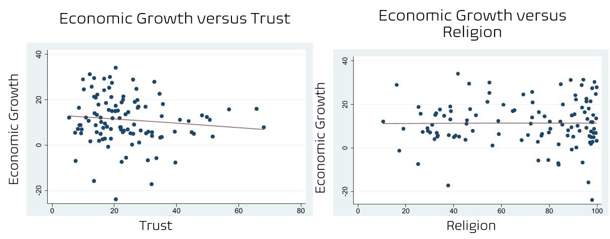 Figure 1: Economic growth versus Trust & Figure 2: Economic growth versus Religion
4
Source: World Values Survey and World Bank
In Figure 3 we see a slight positive correlation between environmental views and economic growth, running counter intuitive to basic common sense and a trade off which nearly all accept as true. When people become more willing to sacrifice economic growth for environmental protections, one would expect that economic growth levels would drop, but this is not the trend observed in this graph nor is this assumption consistent with the results from the model of this study. In Figure 3 we observe a weak but somewhat defined relationship between the two cultural variables of religion and environment. The more defined the relationship between the two cultural variables is, the more interpretable the results of the parameter estimate for their cross variable, as values are more likely to follow a continuous trend that represents a change in both variables.
3.0 LITERATURE REVIEW
3.1 The Effects of Cultural Values On Economic Outcomes
“ Throughout history, one of the defining features of different societies have been the values that they each hold. These values influence every aspect of the culture, including the outcomes that it is capable of producing.
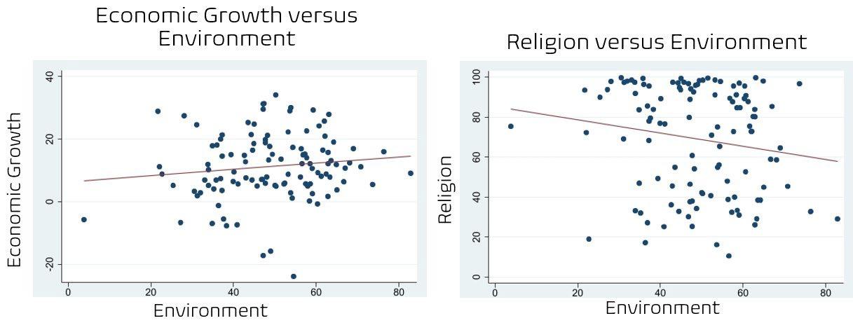 Figure 3: Economic growth versus Environment & Figure 4: Religion versus Environment
5
Values which influence economic outcomes of a nation can be broken down into two categories, individual preferences, which exist at the level of the individual, and political preferences, which reflect attitudes towards the way that government should be run. According to Guiso et al. (2006), “We distinguish between values that influence economic preferences (such as fertility or labor participation preferences) which can be thought of as parameters of a person’s utility function and political preferences (such as preferences for fiscal redistribution). Culture, thus, can affect economic outcomes through both these channels.” Political preferences are likely to reflect the political outcomes of nations, so this variable must be controlled for when analyzing how individual preferences towards women, within a culture, influence economic growth.
Several studies have found connections between cultural backgrounds and types of economic outcomes, including willingness to complete workplace duties. According to Ichino and Maggi (2000), “The prevalence of shirking within a large Italian bank appears to be characterized by significant regional differentials'' . A relationship between shirking and region of origin displays a relationship between an individual's culture and their willingness to work and to what degree that they are willing to do so. Two other studies that also found relationships between cultural attitudes and economic outcomes are from Fernández and Fogli (2005), and Fernández et al. (2004). Fernández et al. (2004) found that men growing up in homes where mothers worked, were significantly more likely to have wives who participated in the labor force. Fernández and Fogli (2005) explored the effects of cultural proxies on first generation immigrants and labor force outcomes for women, using prior women's labor force participation rate and fertility rates as cultural proxies, and economic indicators of women’s labor force participation rate as control variables. These studies found a relationship between past female labor force participation and fertility outcomes with those of modern outcomes, within the same cultural proxies, and the impacts of men growing up with working mothers on female labor participation, respectively.
An additional study from Ferraro and Cummings (2007), found differences in the economic behavior of Navajo and Hispanic groups, including spending, even when controlling for
6
demographic differences, including economic indicators of economic behavior. This study used the ultimatum game, a commonly used tool in behavioral economics, to determine the differences in bargaining behavior between the two ethnic groups. In the ultimatum game, each player is assigned to the role of either proposer or responder, and the proposer is given 10 dollars to split between themselves and the responder, who will decide whether to accept or reject the proposers offer, where rejection leads to an outcome of zero dollars for both players. This study was conducted in Albuquerque, New Mexico with 60 Hispanic participants and 60 Navajo participants. These studies lay the foundation for the claim that economic outcomes are influenced by culture. “ (Barlow 2022).
3.3 Determinants of Economic Growth:
“Measuring economic growth, and determining the factors that contribute to economic growth is a challenge faced by many economists over the past several decades. One of the largest challenges faced is the issue that different countries have different determinants of economic growth. One way economists deal with this issue is by dividing countries into several groups, Developing nations, developed nations, and the nations of SouthEast Asia and Central Europe, which take on a middle ground role between the developed and developing nations.
In a study from Anyanwu (2014), using data from 53 African nations over 3 year periods between 1996 and 2010, and data from China from 1980 to 2010, creates a model of economic growth for developing nations, and compares these factors with the factors that have influenced China’s massive economic growth over a three decade period. The model utilized was a log-log model, with gdp per capita growth as the dependent variable and initial real gdp per capita, government consumption expenditure as a percentage of GDP, the investment rate, official development aid as percentage of GDP, foreign direct investment as a percentage of GDP, total trade a percentage of GDP, external debt as percentage of GDP, secondary school enrolment, inflation rate, institutionalized political regime, government effectiveness, urban population, domestic credit to the private sector as a percentage of GDP, agricultural materials price index, metals price index, oil price
7
index, and the industrial materials price index as independent variables. The study found domestic investment, ODA to GDP, secondary school enrollment, government effectiveness, urban population, and metal price index to be statistically significantly related to GDP per capita growth for the African sample (Anyanwu 2014). When using pooled OLS regression, Domestic investment to GDP, ODA to GDP, secondary education enrollment, gov effectiveness, urban population, and the metal price index to be statistically significantly positively related controls.
In a study from Checherita-Westphal and Rother (2012), using data from 12 countries that use the Euro over the time period from 1970-2008, found that governmental issues, like debt levels, trade openness, and government savings are positively and significantly related to GDP per capita growth for developed nations. The empirical model used for developed nations included GDP per capita growth as the dependent variable, and government debt, government balance, private savings, and trade openness as the independent variables of interest for the study, along with a plethora of economic control variables(ChecheritaWestphal & Rother 2012).
In a study from Fetahi-Vehapi et al. (2015), a model is created to attempt to relate trade openness to economic growth in south eastern European nations, when controlling for other economic variables. The control variables used in this study, when compared to models of economic growth for developing and developed nations, are slightly different as follows; human capital, gross fixed capital formation (GFCF), Active Population, and the FDI (Fetahi-Vehapi et al. 2015). One interesting conclusion of this study to keep in mind is that, population was found to be negatively and significantly correlated with economic growth for these southeastern European countries. The study also found GDP per capita in the prior year, gross fixed capital formation, and human capital to be statically significant and positively related to economic growth.
A study from Barlow (1994) finds no correlation between levels of population growth and economic growth and suggests that there is likely no relationship between the two variables. This study does not explore the relationship when looking at the population
8
growth metrics lagged by the length of a generation, which may have some relationship, given the relationship between increased population and increased human capital.
The theory of convergence, which is suggested by the findings of Barro (2003), suggests that countries with lower GDP per capitas will grow faster than countries with high GDP per capitas. Under this theory, smaller economies will grow at higher rates, relative to their larger economic counterparts, leading to all economies theoretically converging to one size.” Barlow (2023).
3.3 A Note on Environmental Regulation and Economic Growth
Two important studies from Grossman and Krueger (1995) and Jaffe et al. (1995) analyzed the relationship between environmental regulation and a certain contributing factor of economic growth. Grossman and Krueger (1995) analyze the positive relationship between environmental regulation and productivity growth by forcing innovation in capital. Jaffe et al. (1995) analyzed the impacts of the Clean Air Act on innovation in US manufacturing and found that the increased regulation led to increased innovation among firms. It is important to note that each of these studies was only focused inside of the United States.
Despite the conclusions of the previous two studies, a more recent study regarding the economic impacts of environmental regulation comes from Antweiler et al. (2001) This study found that increased environmental regulations culminate in reducing competitiveness and cause businesses to relocate to countries with less environmental regulations in place.
4.0 DATA AND EMPIRICAL METHODOLOGY
4.1 Data
The study uses panel data, based on WVS availability, from 2004 to 2016. Data was obtained from the USAID website IDEA data query system. The summary statistics for both the cultural and economic variables are included below, in Table 1. Note that these summary statistics represent a handful of additional observations that were not utilized in certain models in this study due to a lack of data completeness.
9
Table 1 Summary Statistics
Var N Mean Std. Dev. Min Max Family Importance 116 98.54741 1.49669 87 100 Friends Importance 116 87.69052 8.680443 52.6 98.8 Work Importance 116 88.71638 6.318598 70.8 99.3 Religion Importance 116 69.54569 26.76564 10.6 99.8 Hard-Work-Luck-Scale 113 4.293274 0.9194811 2.12 8.63 Trust 109 23.78073 12.31223 5.4 68.1 Would Serve 116 61.80086 16.94084 15.1 97.8 GDP 114 8.99E+11 2.26E+12 3.16E+09 1.56E+13 GDP (y-1) 114 8.32E+11 2.13E+12 2.89E+09 1.50E+13 Econ Grow 114 11.39599 10.64111 -23.8594 34.16632 Pop Grow 114 1.321661 1.692289 -0.88425 12.72727 Patents Per 100k 96 20.69512 52.41377 0.014635 287.9795 Environment 114 49.07456 13.18656 3.8 82.8 Corruption 114 47.61404 22.84016 16 96 Education 101 80.60396 23.47087 9 100 Infant Mortality 113 19.00885 18.70709 2 92 10
4.2 Empirical Model
This study adapts the standard economic growth model by including potential cultural indicators of economic growth into the model and testing each cross combination for significance. The model utilized in this study has been written below.
Economic Growthit = β0 + β1CulturalVariableit +β2Xit+uit + β3lnGDP(y-1)it + β4PopulationGrowthit + β5Innovationit + β6Corruptionit + β7Educationit + β8InfantMortit + β9CapitalFormationRateit + eit
Economic Growthit is the dependent variable and is measured by the growth rate of GDP from the previous year to this year, with both values measured in 2023 US dollars. The independent variables of interest are all products of two of the cultural variables, all listed below in Table 2.
Table 2 - Cultural Variable Descriptions
Variable Definition
Family Importance % Responded important or rather important to question: “Important in Life: Family”
Friends Importance % Responded important or rather important to question: “Important in Life: Friends”
Work Importance % Responded important or rather important to question: “Important in Life: Work”
Religion Importance % Responded important or rather important to question: “Important in Life: Religion”
Hard-Work-Luck Scale Average of Responses measured on 1-10 scale that “Hard Work Brings Success”; where higher values indicate a view that success is more based on luck
Trust Sum of % responded trust completely and trust somewhat to question: “ Trust: People you meet for the first time”
Would Serve % Would serve for their country's military
Cap Form 106 23.04717 5.625422 12 45
11
Environment
% Believe environment should be given priority over economic growth interests
Source: World Values Survey
Independent control variables consist of seven variables obtained from the World Bank and USAID Query system. First, lnGDP(y-1)it (the natural log of the GDP in the previous year of country i at year t ) represents the size of the economy already present within the nation. PopulationGrowthit (the growth rate of population of country at year ) represents the increase in the workforce. Innovationit (the natural log of the total number of patent applications by residents of country at year ) represents the growth of technology within the country. Corruptionit (perceptions of corruption from transparency international of country at year ) represents the level of political corruption in a country, higher levels indicate less corruption. Educationit (the percentage of individuals who have completed secondary school of country at year) represents the average level of education in the nation. InfantMortit (the number of deaths per 1,000 live births of country at year ) represents the quality and accessibility of healthcare within the country. Finally, CapitalFormationRateit (the gross fixed capital formation rate as a percentage of GDP of country at year ) represents the investment into new non-human capital.
5.0 EMPIRICAL RESULTS
The empirical estimation results are presented in Table 3. The primary results displayed relationships between religiosity and environment and the dependent economic growth variable. The results of each of these regressions along with the cross variable, enviroreligion, which is a product of the two variables, are displayed below. In order to determine the success of the cross variable, we must see if the adjusted r squared raises to a significant degree from the two solo variable models. As we see in Table 3, the adjusted R-squared is the highest in model III, at .6606, but this is not enough of a difference from the adjusted R-squared’s found in model I and II respectively, at .6274 and .6595, to conclude that this difference would continue to be accurate using a larger data se


Table 3: Regression results
12
Economic Growth
Note: *** , **, and * denotes significance at the 1%, 5%, and 10% respectively. Standard errors in parentheses
Variables I Religion II Environment III Cross Religion Importance .6343** (.2424) Environment .4719*** (.102) EnviroReligion Cross .0061** (.0025) ln(GDP (y-1)) -3.0144 (5.1239) -6.5393 (6.1745) -2.5852 (6.0256) Pop Grow 3.097 (3.3877) .8029 (3.9241) 1.3526 (3.9868) Innovation -.2194*** (.0706) -.2972** (.1133) -.2335*** (.0869) Corruption -.5364 (.3686) -.3796 (.4323) -.4244 (.4085) Education .1153 (.2227) .1040 (.1581) .0572 (.1839) Infant Mort 1.4777*** (.4929) 1.3246** (.6432) 1.6877*** (.6265) Capital Formation .6896 (.4406) .1840 (.5706) .2489 (.5277) R2 0.6274 0.6595 0.6606 F-statistics 17.38*** 9.59*** 12.33*** Number of obs. 87 87 87
13
Both the religion and environment variables were found to have significance in their respective models at the 1% level. In the case of Religion, this parameter estimate displays a relationship in the same direction as Barro & McCleary (2003), showing that increased intensity of religious beliefs leads to higher levels of economic growth, ceteris paribus. The parameter estimate for the environmental belief factor is positive, displaying a positive relationship to economic growth, running contrary to the idea of the environmental-economic trade off suggested in Antweiler et al. (2001). This positive parameter estimate also is not accounted for by the results found in Grossman and Krueger (1995) and Jaffe et al. (1995), as these models all control for the innovation variable. The cross variable, Enviro-religion, analyzed in model three, is significant at the 5% level.
The natural log of GDP in the prior year was not found to be significant in any of the three models, which goes against the theory of convergence proposed in Barro (2003). Population growth was not found to have significance in any of the three models, although a larger population lag, longer than a year, was not utilized. This finding aligns with the findings of a study from Barlow (1994).
The innovation variable was found to be significant in all three models with a negative parameter estimate, at the 1%, 5%, and 1% level respectively. This parameter estimate directly contradicts the findings of Fetahi-Vehapi et al. (2015), who found a positive relationship between patent applications and economic growth. Both corruption and education were found to be insignificant in all of the regressions. Infant Mortality was found to be significant in all three models at the 1%, 5% and 1% level, respectively, with positive parameter estimates. The sign of this parameter estimate is counter intuitive to economic growth, but may have some relationship to the idea of convergence with more developed nations growing slower. Capital formation was not found to be significant in any of the models which contradicts the findings of FetahiVehapi et al. (2015), who found that capital formation rate was an important indicator of economic growth.
14
5.0 CONCLUSION
This study aims to expand upon the existing literature regarding the impacts of cultural values on economic growth by analyzing the effects of several cultural factors working together in one quantifiable variable. The major contribution of this study is the positive relationship discovered between positive attitudes towards the environment and economic growth. This relationship suggests that environmental protection may not have to come at the cost of positive economic outcomes, which could prove extremely beneficial to human society.
Policy makers should look to apply this study in informing policy decisions regarding environmental regulation of businesses. Protecting the environment is not found to have a negative relationship with economic growth in this study and therefore, environmental regulation may not be as harmful to the economy of a nation as previously estimated.
The major limitation of this study was the lack of availability of cultural variables due to the structure of the World Values Survey. Future research should look to analyze an increased number of cultural-cross variables, which quantify more than one cultural attitude. In addition, future studies should further explore the depth of certain cultural factors and their own individual aspects, to avoid oversimplification of factors like intensity of religious beliefs, or the importance of work and family in your life, etc.
15
Appendix A: Variable Description and Data Source
Acronym Description
Family Importance
Friends
Importance
Work Importance
Religion
Importance
% Responded important or rather important to question: “Important in Life: Family”
Data source
World Values Survey
% Responded important or rather important to question: “Important in Life: Friends”
% Responded important or rather important to question: “Important in Life: Work”
% Responded important or rather important to question: “Important in Life: Religion”
Hard-Work-Luck Scale Average of Responses measured on 1-10 scale that “Hard Work Brings Success”; where higher values indicate a view that success is more based on luck
Trust
Sum of % responded trust completely and trust somewhat to question: “ Trust: People you meet for the first time”
Would Serve
World Values Survey
World Values Survey
World Values Survey
World Values Survey
World Values Survey
% Would serve for their country's military World Values Survey
Environment
% Believe environment should be given priority over economic growth interests
GDP
GDP
World Values Survey
World Bank
16
GDP (y-1) GDP in the previous year
Econ Grow
Change in GDP from previous to current year
Pop Grow
World Bank
calculated
Change in population from previous to current year calculated
Patents Per 100k The number of patent applications by residents per 100k residents
Corruption The levels of corruption present in the nation (higher is less corrupt)
Education % of people who completed secondary school
Infant Mortality number of infant deaths per 1,000 live births
Cap Form gross fixed capital formation rate
World Bank
Transparency international
World Bank
World Bank
World Bank
17
Acronym
Religion
Appendix B- Variables and Expected Signs
% Responded important or rather important to question: “Important in Life: Religion”
Average intensity of religious beliefs +
Environment
% Believe environment should be given priority over economic growth interests
Percentage believe in environment over economic interestsReligion-enviro
product of the Religion and Environment variables.
GDP (y-1)
in the previous year The size of the country’s economy in the previous year
Econ Grow Growth rate of GDP from previous year to year of survey
Pop Grow Growth rate of population from previous year to year of survey
Patents Per 100k
The growth of the nations economy
Increases in human capital +
The number of patent applications by residents per 100k residents Innovation levels +
it captures Expected sign
Variable Description What
cross
Represents
+/GDP GDP
the
economy N/A
The
a relationship between the two variables
The size of
country’s
GDP
-
N/A
18
Corruption
Average perceptions of levels of corruption
Education
% of people who completed secondary school
Infant Mortality number of infant deaths per 1,000 live births
Cap Form gross fixed capital formation rate
The levels of corruption present in the nation (higher is less corrupt)
Average levels of education +
Proxy for average quality of healthcare -
the increase in non human capital +
+
19
Anyanwu, J. C. (2014). Factors affecting economic growth in Africa: Are there any lessons from China? African Development Review 26(3), 468-493.
Antweiler, W., Copeland, B. R., & Taylor, M. S. (2001). Is free trade good for the environment? American Economic Review, 91(4), 877-908.
Barlow, J (2023). Economic Growth and Cultural Attitudes Towards Women: An Empirical Investigation. [Unpublished honors thesis]. Bryant University.
Barlow, R. (1994). Population Growth and Economic Growth: Some More Correlations. Population and Development Review, 20(1), 153–165. https://doi.org/10.2307/2137634
Barro, R.J. (2003). Determinants of economic growth in a panel of countries. Annals of Economics and Finance 4, 231–274. http://down.aefweb.net/WorkingPapers/w505.pdf
Checherita-Westphal & Rother. (2012). The impact of high government debt on economic growth and its channels: An empirical investigation for the Euro area. European Economic Review 56, 1392-1405.
Fernández, R., Fogli, A., & Olivetti, C. (2004). Mothers and sons: Preference formation and female labor force dynamics. Quarterly Journal of Economics, 119(4), 1249 –99.
Fernández, R & Fogli, A. (2005). Culture: An empirical investigation of beliefs, work, and fertility. American Economic Journal: Macroeconomics, American Economic Association, 1(1), 146-177. https://ideas.repec.org/a/aea/aejmac/v1y2009i1p146-77.html
Ferraro, P. & Cummings, R. (2007). Cultural diversity, discrimination, and economic outcomes:
BIBLIOGRAPHY
20
An experimental analysis. Economic Inquiry, 45(1), 217-232. https://doi.org/10.1111/j.14657295.2006.00013.
Fetahi-Vehapi, Sadiku, & Petkovski. (2015). Empirical analysis of the effects of trade openness on economic growth: An evidence of south east European countries. Procedia Economics and Finance 19, 17-26.
Grossman, G. M., & Krueger, A. B. (1995). Economic growth and the environment. The Quarterly Journal of Economics, 110(2), 353-377.
Guiso, L., Sapienza, P., & Zingales, L. (2006). Does culture affect economic outcomes? Journal of Economic Perspectives, 20(2). 23-48.
Ichino, A. & Maggi, G. (2000). Work environment and individual background:
Jaffe, A. B., Peterson, S. R., Portney, P. R., & Stavins, R. N. (1995). Environmental regulation and the competitiveness of US manufacturing: What does the evidence tell us? Journal of Economic Literature, 33(1), 132-163.
Explaining regional shirking differentials in a large italian firm. Quarterly Journal of Economics, 115(3). 1057–90.
21
Fenway and Crime: Opportunity, Geographic Differences, and Team Rivalry at Boston Red Sox Games
Cole McGovern
Abstract:
Although hosting professional sports are often seen as a financial benefit for cities, there are also associated costs. This paper investigates the possibility of interdependence between a variety of crimes and home game days of the Boston Red Sox. When adjusting for game attendance and length, minor assaults charges such as disorderly conduct and simple assault increase city-wide during game days. Despite this, all crime around the immediate stadium area decreases in volume. Additionally, this study examines differences in geographical impacts and crime levels, when a game was played, and games played against the New York Yankees, their historic rival
JEL Classification: L83, R23, Z21
Keywords: baseball, MLB, Boston, crime, team rivalry
Bryant University, 1150 Douglas Pike, Smithfield, RI02917. Phone: (860)-942-3918.
Email: cmcgovern3@bryant.edu.
22
1.0 INTRODUCTION
While Major League Baseball (MLB) has generally been seen as a family friendly sport, not many previous studies have not investigated the link between crime and hosting a professional baseball game. Several studies, however, have linked football and soccer to increasing crime rates. This gap in literature could be the result that baseball is considered a family friendly spectator sport and not associated with rioting sometimes seen during soccer or college football games (Seff, 2015). However, MLB games may result in an increase in crime due to a larger attendance and increased opportunity.
This study aims to enhance the overall understanding of professional sports impact on crime rates. From a policy perspective, this analysis is important because could lead to better crime prevention policies and programs to reduce crime caused by sports. Using nearly five years of daily data from Boston, MA, we examine how crime rates are likely to change in Boston during Red Sox game days.
Crimes are examined based on likely perpetrators (disorder offenses) and likely victims (pecuniary offenses). An opportunity variable also considers attendance and game length in attempts to measure the elasticity of the crime during game time. Results indicate that Boston Red Sox games are likely responsible for increases in all common crime rates in Boston by 2.38%, Disorderly Conduct by 18.95%, and Simple Assault Charges by 6.67%.
When analyzing the impact by district, all crime in the districts surrounding Fenway Park decreased by 1.5%. Robbery also decreases by 6.5%, and Burglary by 16.8% in the immediate stadium area. When playing against teams that aren’t the New York Yankees, city-wide crime reduces by 0.95% and Burglary also decreases by 4.31%. Day games reduce city-wide Burglary by 4.94%.
This paper was guided by three research objectives: First it investigates the possibility of interdependence between game days and city-wide crime using time-series data; Second, it incorporates the opportunity-proxy model to examine the influence of location on crime; We also utilize the opportunity-proxy model to examine the impact of games against rival teams and the time of the games impact on city-wide crime. Although there has been similar
23
empirical work done in the past, no previous literature has examined a city with such a relatively low crime rate such as Boston. This paper successfully fills this void.
The rest of the paper is organized as follows: Section 2 provides an overview of trends. Section 3 gives a brief literature review. Section 4 outlines the empirical model, data, and estimation methodology. Finally, section 5 presents and discusses the empirical results. This is followed by a conclusion in section 6.
2.0 TRENDS OF BOSTON CRIME
Figure 1 shows that from 2003 to 2018, the crime rate in Boston has been on a clear downward trend with a significant decrease in the number of violent crimes. Although the national crime rate has also decreased during the same period, Boston’s crime rate has dropped relatively more. According to the Boston Police Department, the city's crime rate has dropped more than 25% since 2010. In contrast, the national crime rate has only decreased by less than 10% since. The decrease in the national crime rate can likely be attributed to improving economic conditions reducing poverty. The decrease in Boston can likely be attributed to increased policing efforts throughout the city.
Source: Federal Bureau of Investigation’s Uniform Crime Reports
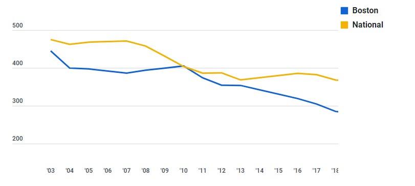 Figure 1: Violent Crime Rate (Boston/National)
24
Figure 2 shows that from 2016 to 2019, crime rates in Boston for some of the UCF Part I crimes such as Robbery, Burglary, Motor Vehicle Theft, Vandalism, and Disorderly Conduct have been massively trending downward. Since 2016, Robbery has decreased by 36.6%, Burglary by 32.7%, Motor Vehicle Theft by 23.6%, Vandalism by 29.8%, and Disorderly Conduct by 71.6%. Property crime in Boston has been occurring at a decreasing rate.
Figure 3 shows that from 2015 to 2020, the incident daily average for all crimes in Boston are higher on game days. Although Boston's crime rate has decreased significantly over the past decade, the city still faces significant challenges in reducing crime. For example, some districts have historically experienced higher levels of violence. Crime rates can also vary widely from one year to the next. As a result, it is important to examine long-term trends to get a more accurate picture of the overall trajectory of crime in each area.
Figure 2: Boston Yearly Crime Totals
Source: Boston Police Department
0 1000 2000 3000 4000 5000 6000 2016 2017 2018 2019 Robbery Burglary Motor Vehicle Theft Vandalism Disorderly Conduct 25
Incident Daily Average
Source: Boston Police Department
3.0 LITERATURE REVIEW
The relationship between sports and higher levels of crime can be explained by the team rivalry, alcohol consumption, disappointment over the game result, and an increased opportunity to commit during game times. When examining previous literature, violent crimes and aggressive behavior have been connected to European soccer. Ward (2002) suggests that the lower levels of violence in the United States are result of the lower popularity of soccer and a more diverse base of spectators. Marie (2016) finds a significant relationship between attendance and crime, with about a 4% increase in crime for each 10,000 attendees at a soccer match. In European soccer, a fan’s allegiance to a team is typically determined by where they grew up or familial ties Since professional teams in the United States typically have a shorter history when compared to European soccer and don’t have as much of a local pull when compared to soccer. Roberts and Benjamin (2000) state that, “The idea of Manchester United being ‘sold’ to another city is unthinkable in the United Kingdom”. However, teams are frequently sold in the United States.
Although the lack of deep team rivalries in the United States may be an outcome of the mobility of professional sports teams, violence and aggression have still been common enough make policing at sports events extremely challenging (Madensen & Eck, 2008). Roberts and Benjamin (2000) also believe that sports with highly violent player behavior
Figure 3: Incident Daily Average (Game Day/Non-Game Day)
0 10 20 30 40
Robbery Aggrivated Assault Burglary Larceny Motor Vehicle Theft Vandalism Disorderly Conduct Simple Assault
26
Game Day (n = 369) Non-Game Day (n = 1367)
reflect onto their spectators. For example, sports such as American football and hockey in the United States are often seen to have high levels of unpunished violence on the field. Whereas European soccer or basketball games highly regulate violent player behavior. Since baseball is a sport that highly regulates violent player behavior, we should expect to see less assault charges at MLB games when compared to other sports. On the other hand, MLB games may yield higher rates of aggressive spectator behavior because baseball is one of the oldest professional sports in the United States. Baseball is considered to be “Americas Game” and many teams in the MLB have historical roots dating before the 19th century. This makes it by far the oldest popular sport in the United States. Only a limited amount of MLB teams relocate when compared to other leagues like the NFL or NBA, which may explain why higher levels of historical team rivalries exist in the MLB. Due to this high amount of team rivalry in MLB, we should expect to see higher crime rates on games played against a rival team
When examining the levels of alcohol consumption at sports games, there has been an established connection between alcoholic intake and increased criminal behavior. Some increased behavior includes assaultive behavior, property damage, and vandalism (Boden, Fergusson, & Horwood, 2013; Ostrowsky, 2014). Card and Dahl (2011) also find that crime may not just increase in the immediate stadium area, but that spectators in a variety of locations may be impacted due to a big win or loss One sample found that 60% of males ages 20-35 at an MLB are likely to show evidence of alcohol consumption. By the fifth inning, 13% were legally impaired (Wolfe, Martinez, & Scott, 1998). When combining this information with evidence of excessive alcohol consumption leading to lower self-control and the large amount of people in a concentrated area, we should expect to see an increased rate of aggressive behavior at MLB games.
Cohen and Felson in 1979 developed the Routine Activities Theory (RAT). RAT useful to explain the framework of the opportunity for crime. Despite declining poverty rates in the 1970s, property offenses in the United States increased. Homes were becoming increasingly suitable targets for burglaries as supervision was reduced. This is a result of an increased female participation in the labor market, reducing neighbor supervision.
27
According to Cohen and Felson (1979), crimes occur when three elements are fulfilled: there is a motivated offender, a suitable target, and a lack of supervision. The likelihood of crime occurring can change depending on the supply of opportunities. Relating this information to professional sports games, the supply of suitable targets increases as their property is unsupervised MLB teams average around 30,000 spectators per game and the majority travel by vehicle (Humphreys & Pyun, 2018). Vehicles likely sit concentrated in parking garages and unattended during games. Those who arrive late often must park on side streets and areas with even less supervision. Spectators who live outside the area may not be very familiar with local crime patterns. Many attendees may not take typical precautions that many locals may take, such as putting valuables out of sight. The average MLB also game lasts over 3 hours and parking garages and streets heavily unsupervised. All these factors make spectators at MLB games suitable targets to be victims of crime.
Although Baumann, Ciavarra, Englehardt, and Matheson (2012) found no evidence of professional sports teams leading to increased property or violent crimes, prior studies have found that robberies increase during NBA games and street crimes focused on pecuniary gain are likely to increase because a greater number of targets present themselves in a highly concentrated area. (Yu, McKinney, Caudill, & Mixon, 2016). We also must consider the time at which the game is played. Games played during evening hours may provide an increase in opportunities due to the darkness reducing supervision. This will likely increase the rate for property offenses, but likely won’t impact fan behavior. Alcohol use can also increase the risk of theft as it reduces a person’s situational awareness All these factors may lead them to become easy victims of theft or robbery. Rees and Schnepel (2009) concluded that home College football games are associated with a 9% increase in Assaults, 18% increase in Vandalism, 13% increase in DUI’s, and a 41% increase in Disorderly Conduct charges. However, away games did not significantly affect local crime levels. As a result, we should expect that property offenses, especially those focused on vehicles, are likely to increase during MLB game days.
It is important to note that the Red Sox provide additional security by hiring off-duty police officers and the city increases supervision around the stadium during game days, especially
28
against rival teams. Even an increase in crime around the stadium may not lift city crime levels if local offenders purposively travel to the stadium area to commit offenses. As a result, it will require a substantial increase in crime around the stadium area on game days to significantly change citywide crime levels in a big city such as Boston. Overall, we expect that property crime levels (such as larceny and motor vehicle theft) and minor aggressive offenses directly around Fenway Park will increase during game days
4.0 DATA AND EMPIRICAL METHODOLOGY
4.1 Data
The study uses annual data time-series data from 2015 to 2020. Boston daily crime data was collected from Boston Police Department of Innovation and Technology. Data was collected as far back as they offered (June 15th, 2015) to the date before the United States lockdown for COVID-19 (March 13th, 2020). The Boston Police Department uses Uniform Crime Reporting (UCR) to ensure a degree of consistency in recording crime All major crime categories (Part I crimes) were examined in this study as they report a reasonable daily frequency. For example, homicide is not considered to be a part of Part I crimes as they rarely occur at a daily level. All Part I crimes include robbery, aggravated assault, burglary, larceny, and motor vehicle theft, simple assault, disorderly conduct, and vandalism.
Boston was mainly selected due to the availability of their data. However, they have a relatively low crime rate when compared to other major cities. Although another study has analyzed the impact on a city with high crime rates, St. Louis, nobody has analyzed a city with lower crime rates to compare results. The Boston Red Sox are one of the main teams in the MLB due to their long history and loyal local fan base. This ensures a consistent high attendance and heated rivalry games against the New York Yankee’s. The average attendance at Red Sox games is slightly above 36,000 per game.
Instead of using distance bands, we group crime into four categories based on their relationship to Fenway Park: Fenway, Near Fenway, City Center, and City-Wide. Crime will be grouped into Fenway if it occurs in Fenway/Kenmore (D-4). Near Fenway if it
29
occurs in Allston/Brighton (D-14), Mason Hill/Roxbury (B-2), South Boston (C-6), and City Center (A-1). City center if occurs in A-1 and all districts if occurred city-wide. See Figure 4 for more information on district layouts in Boston.
Source: ResearchGate
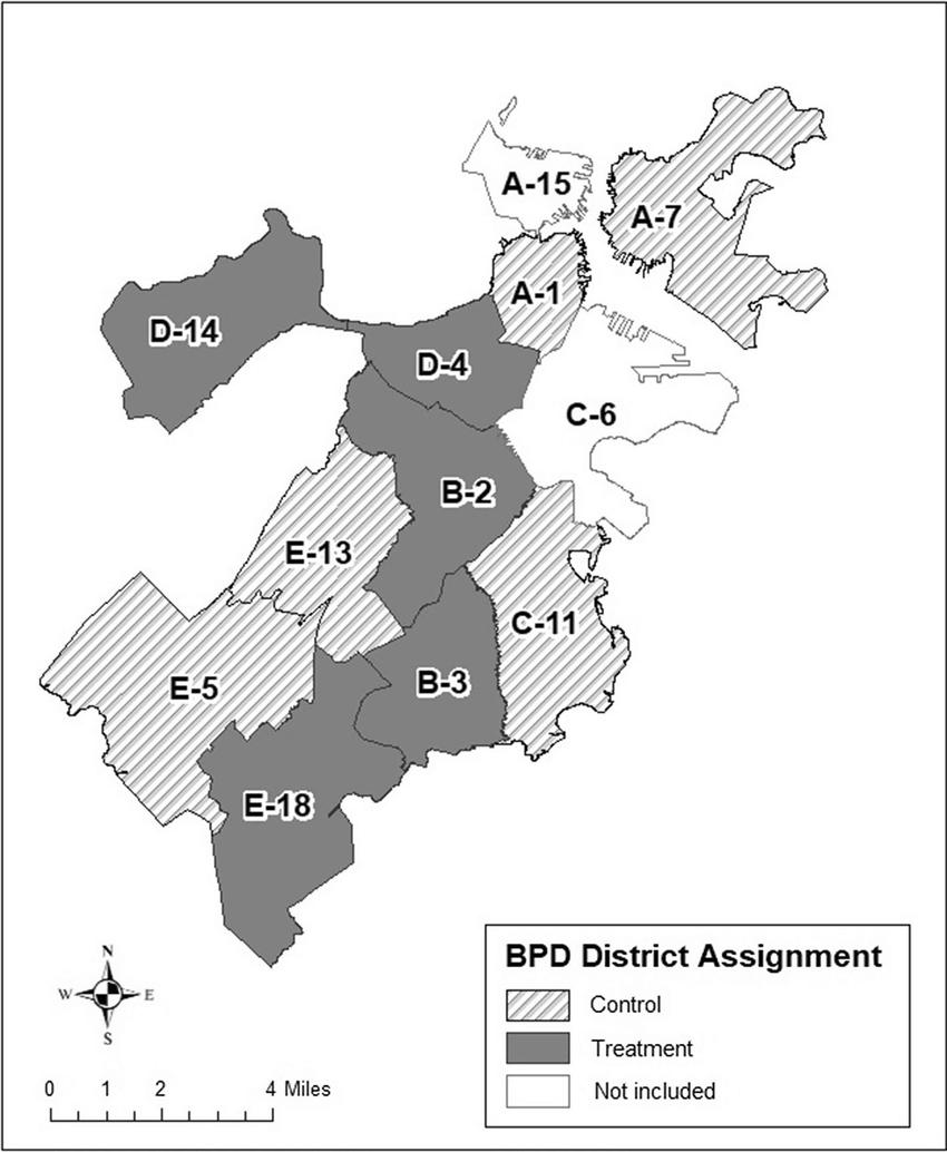 Figure 4: Boston District Map
30
The Red Sox play schedule was retrieved from Baseball-Reference as they post historical MLB schedules (https://www.baseball-reference.com). Included are the game dates, the name of the opposing team, whether a play occurred home or away, whether the game was played at day or night, attendance numbers, and game duration. Both regular season and postseason games are included. Home game days for the two other professional sports teams in Boston, the Celtics (NBA) and the Bruins (NHL) act as control variables. We generated binary variables for all home games for MLB, NHL and NFL games.
Because previous studies have found that daily crime counts are impacted by climatic variation such as Cohn & Rotton (2000), the current study includes a variety of weather data such as precipitation, snowfall, temperature, windspeed, hail, fog, and thunder. Daily climate data was collected from the National Oceanic and Atmospheric Administration at Boston Logan International Airport. Logan is located roughly 5.6 miles away from Fenway Park and has some of the most accurate weather data in the region.
Additional control variables are generated to account for time-varying influences on crime. Most daily crime studies incorporate binary indicators for federal holidays such as Cohn & Rotton (2003). Summary statistics for the data are provided in Table 1.
31
Table 1 Summary Statistics
4.2 Empirical Model
The analytical strategy of this study rests on time-series modeling. The distribution of crimes counts in our data was nonnormal due to the low frequency at which crimes occur on a daily level. Since most of the variables have a higher standard error when compared to their mean, a Negative Binomial Generalized Linear Model (GLM) employing a log link must be used instead of a traditional OLS regression.
Variable Observation Mean Std. Dev. Min Max Opportunity 454 7.21 1.467 4.73 16.82 RedSoxHome 1738 0.212 0.409 0 1 CelticsHome 1738 0.010 0.101 0 1 BruinsHome 1738 0.127 0.333 0 1 Precipitation 1738 0.118 0.294 0 2.7 Snowfall 1738 0.107 0.786 0 14.5 Temperature 1738 47.416 15.947 0 108 Temperature2 1738 2502.449 1475.542 0 11664 Windspeed 1738 11.059 3.827 3.2 38.1 Hail 1738 0.005 0.072 0 1 Fog 1738 0.083 0.276 0 1 Thunder 1738 0.047 0.212 0 1 Holiday 1738 0.031 0.174 0 1 AllP1 1738 73.932 15.62 0 133 Robbery 1738 3.534 2.15 0 12 Aggravated Assault 1738 6.473 2.99 0 23 Burglary 1738 5.665 3.06 0 20 Larceny 1738 30.372 7.70 0 58 Motor Vehicle Theft 1738 3.819 2.27 0 14 Vandalism 1738 11.845 4.72 0 35 Disorderly Conduct 1738 0.939 1.08 0 8 Simple Assault 1738 13.285 4.48 0 39 32
We modify Mare & Blackburn’s (2019) model on baseball affecting citywide crime as shown:
Ln E (crimet) = τt + β0 + β1RedSoxHomet + β2CelticsHomet + β3BruinsHomet + β4Precipitationt + β5Snowfallt + β6Temperaturet + β7Temperature2t + β8Windspeedt + β9Hailt + β10Fogt + β11Thundert + β12Holidayt + ε
The equation above describes that the expected level of crime at day (t) is the predicted outcome of: Binary variables for Boston Red Sox home games (RedSoxHome), Boston Celtics home games (CelticsHome), and Boston Bruins home games (BruinsHome). Weather controls such as precipitation (in), snowfall (in), temperature (F), a squared temperature term to account for the nonlinear effects of temperature, and windspeed (MPH). Lastly, binary variables that may impact game attendance (hail, fog, thunder). Federal holidays are also included as per Cohn & Rotton (2003).
Mare & Blackburn’s (2019) study also include an opportunity variable in attempts to capture the elasticity of crime:
The goal of the opportunity variable is to capture the changing crime opportunities on a game day (t) which are measured as the result of which the Red Sox either play at home (1) or do not play a home game (0) multiplied by attendance and game length (in minutes). Although not every additional attendee or minute of game creates an actual crime opportunity, it may increase the chance of a crime being committed. Although output is not listed due to the lack of significant results, models for Table 2 were also run using the opportunity variable.
33
5.0 EMPIRICAL RESULTS
The empirical estimation results for game days and city-wide crime are presented in Table 2. The empirical estimation shows that when the Red Sox play at home, city-wide common crime rates in Boston increase by 2.38% with significance at the 5% level, Disorderly Conduct increases by 18.95% with significance at the 1% level, and Simple Assault Charges by 6.67% with significant at the 1% level
34
Table 2: Game Day and City-Wide Crime
Note: ***, **, and * denotes significance at the 1%, 5%, and 10% respectively. Standard errors in parentheses
The empirical estimation results for game days and geographic crime differences are presented in Table 3 The empirical estimation shows that all crime in the districts surrounding Fenway Park decreased by 1.5% with significance at the 10% level. Robbery also decreases near Fenway by 6.5% with significance at the 10% level. Burglary
Dependent Variables All Part 1 Crimes Robbery Aggravated Assault Burglary Larceny Motor Vehicle Theft Vandalism Disorderly Conduct Simple Assault RedSoxHome 0.0237 (0.0116)** -0.0284 (0.0391) 0.0377 (0.0275) -0.0452 (0.0335) 0.0122 (0.0148) 0.035 (0.0354) 0.0246 (0.0246) 0.1895 (0.0699)*** 0.0667 (0.0205)*** CelticsHome -0.0777 (0.0445)* -0.1422 (0.1567) -0.0607 (0.1059) -0.1153 (0.1345) -0.1475 (0.0587)** -0.0611 (0.1429) 0.0252 (0.0922) -0.1735 (0.2765) -0.0067 (0.0753) BruinsHome 0.0065 (0.0136) 0.0019 (0.046) 0.0176 (0.0335) -0.0543 (0.0407) 0.0271 (0.0174) -0.0204 (0.0449) -0.0353 (0.0294 -0.0409 (0.0903) 0.027 (0.0247) Precipitation -0.0595 (0.017)*** 0.0291 (0.0561) -0.0913 (0.0421)** 0.0116 (0.0459) -0.0514 (0.0219)** -0.0287 (0.0544) -0.1114 (0.0366)*** 0.0093 (0.1041) -0.0926 (0.0317)*** Snowfall -0.0253 (0.0066)*** 0.0005 (0.0218) -0.0111 (0.017) -0.0354 (0.0212)* -0.0437 (0.0092)*** 0.0272 (0.0207) -0.0149 (0.0139) -0.0141 (0.0428) -0.0353 (0.0129)*** Temperature 0.0099 (0.0015)*** 0.0139 (0.0053)** * 0.0167 (0.0039)*** 0.0092 (0.0045)** 0.0072 (0.0019)*** 0.0019 (0.0049) 0.0135 (0.0033)*** 0.0305 (0.0108)*** 0.0116 (0.0028)*** Temperature2 -0.00004 (0.00001)*** -0.0001 (0.0001)* -0.0001 (0.0001)** -0.0001 (0.0001) -0.0001 (0.0001) 0.0001 (0.0001) 0.0001 (0.0001)** 0.0002 (0.0001)** 0.0001 (0.0001)*** Windspeed -0.0028 (0.0012)** -0.0072 (0.0041)* -0.0046 (0.003) -0.0059 (0.0035)* -0.0053 (0.0015)*** -0.0107 (0.0039)*** 0.0041 (0.0026) 0.0031 (0.0078) 0.0017 (0.0022) Hail -0.0928 (0.0637) -0.0507 (0.2135) 0.1199 (0.1518) 0.0362 (0.1535) -0.123 (0.054) -0.2535 (0.2347) -0.226 (0.1446) -0.5539 (0.5276) -0.0147 (0.116) Fog -0.0124 (0.0174) -0.0551 (0.0592) 0.0171 (0.0418) -0.0516 (0.051) -0.0035 (0.0222) -0.1577 (0.0572)*** 0.0306 (0.0365) 0.0743 (0.1071) -0.0123 (0.0319) Thunder -0.0935 (0.022) -0.0323 (0.0741) -0.0552 (0.0559) -0.0419 (0.0635) -0.0051 (0.028) -0.0369 (0.0672) -0.0045 (0.0466) 0.0592 (0.1314) 0.0072 (0.0399) Holiday -0.0995 (0.0255)*** -0.0557 (0.056) 0.1004 (0.0559)* -0.2193 (0.0783)*** -0.1922 (0.034)*** -0.0251 (0.0502) 0.0073 (0.0532) 0.0505 (0.1564) -0.0655 (0.0701) 35
decreases by 16.8% in the immediate stadium area with significance at the 10% level. Other significant variables include Celtics games reducing city-wide crime by 7.78% with significance at the 10% level and city-wide Larceny by 14.75% with significance at the 5% level. All weather variables showed some form of significance with worse weather decreasing crime rates. Lastly, federal holiday’s decreases the likelihood of property crimes such as Burglary and Larceny.
Note: ***, **, and * denotes significance at the 1%, 5%, and 10% respectively. Standard errors in parentheses
Dependent Variables Fenway Near Fenway City Center All Part 1 Crimes -0.0130 (0.0114) -0.0155 (0.0081)* -0.0154 (0.0147) Robbery 0.0112 (0.0492) -0.0658 (0.0357)* 0.0102 (0.058) Aggravated Assault -0.0559 (0.0475) -0.0068 (0.0244) -0.0274 (0.0516) Burglary -0.1681 (0.0662)** -0.0442 (0.0289) -0.0671 (0.0721) Larceny 0.0159 (0.0147) -0.0199 (0.0124) -0.0303 (0.0193) Motor Vehicle Theft -0.0609 (0.0583) 0.0086 (0.0345) 0.0365 (0.0667) Simple Assault 0.0374 (0.0252) -0.0053 (0.0164) -0.0094 (0.031) Vandalism 0.0206 (0.034) -0.0027 (0.0197) 0.0153 (0.0411) Disorderly Conduct -0.0661 (0.0861) -0.0032 (0.0568) 0.0912 (0.0735)
Table 3: Geographic and Crime Differences, Game Day Coefficients Only
36
The empirical estimation results for game days and geographic crime differences are presented in Table 4. The empirical estimation shows that when playing against teams that aren’t the New York Yankees, city-wide crime in Boston reduces by 0.95% with significant at the 10% level. Burglary also decreases city-wide by 4.31% with significant at the 10% level These estimates are inconsistent with Mare & Blackburn’s (2019) results as crime in the immediate area around the stadium is expected to increase.
Note: ***, **, and * denotes significance at the 1%, 5%, and 10% respectively. Standard errors in parentheses
The empirical estimation results for game days and geographic crime differences are presented in Table 5 The empirical estimation shows that day games reduce city-wide Burglary by 4.94% with significant at the 10% level. This estimate is inconsistent with previous literature as there are a lack of significant connecting night games to increased property crime.
Table 4: Team Rivalry—Red Sox Versus Yankee’s—Game Day Coefficients Only.
Dependent Variables All Part 1 Crimes Robbery Aggravated Assault Burglary Larceny Motor Vehicle Theft Simple Assault Vandalism Disorderly Conduct Yankee’s 0.0131 (0.0118) .0044 (.0557) -0.0226 (0.0429) -0.0144 (0.047) 0.0212 (0.0198) -0.0262 (0.0534) 0.0225 (0.0286) 0.0426 (0.0286) -0.2103 (0.1311) Other teams -0.0095 (0.0055)* -.0397 (.0255) -0.0016 (0.0166) -0.0431 (0.0221)* -0.0127 (0.008) 0.0045 (0.0224) 0.0066 (0.0117) -0.0069 (0.0148) -0.0017 (0.043) 37
Table 5: Time of Day—Night Versus Day Games—Game Day Coefficients Only.
Note: ***, **, and * denotes significance at the 1%, 5%, and 10% respectively. Standard errors in parentheses
6.0 CONCLUSION
Although our study did not find significant evidence, such as Mare & Blackburn’s (2019) study, that home games result in an increase of expected property crimes, we did find a significant relationship between home games resulting in an increase of expected minor assault charges (Disorderly Conduct and Simple Assault). Boston also had a much lower expected increase in common crime when compared to Mare & Blackburn’s (2019) study performed on St. Louis (15%).
Policy to reduce MLB games impact on crime should focus primarily on crowd control in the immediate stadium area to reduce the Disorderly Conduct and Simple Assault charges around the stadium. Regulations related to alcohol sales at games will likely reduce the likelihood of minor assault charges. We also echo Mare and Blackburn’s (2019) recommendations on increasing surveillance on parked vehicles since they appear to be at especially high-risk during games. Alerting spectators to park vehicles in well-supervised areas and to hide personal belongings may decrease property crimes on game days.
The main limitation of this study relates to the credibility of city-wide results. Boston is a large city that constantly hosts other events that could result in increases in crime. Trying to account for all variables affecting city-wide crime is nearly impossible and must be
Dependent Variables All Part 1 Crimes Robbery Aggravated Assault Burglary Larceny Motor Vehicle Theft Simple Assault Vandalism Disorderly Conduct Day game -0.0057 (0.0088) -0.0516 (0.0441) 0.0060 (0.0282) -0.0494 (0.0299)* 0.0011 (0.0129) 0.0056 (0.0362) 0.0109 (0.0182) -0.0112 (0.0232) -0.1079 (0.0781) Night game -0.0083 (0.006) -0.0274 (0.0268) -0.0063 (0.0188) -0.0419 (0.0262) -0.0155 (0.0094) 0.001 (0.0254) 0.0067 (0.0133) 0.0059 (0.0161) 0.0226 (0.0479) 38
assumed to occur randomly on game days and non-game days. As a result, the true impact of MLB games on crime could be much higher as analyzing the city-wide impact can reduce game effects to such small levels. Another limitation of the study is that cities and MLB teams and cities keep their police and security staffing private, so including it as a control variable is nearly impossible. However, we do know that the Boston Red Sox increase security on game days, especially for rival games against the Yankee’s.
Although more analysis is needed, Boston’s lack of an increase in property crimes on game days is likely result of having stronger surveillance over personal property and should be strived to be replicated in other major cities.
39
Appendix A: Variable Description and Data Source
Acronym Description
Opportunity Proxy variable calculated based on game attendance & length
Data source
RedSoxHome Binary variable for when Boston Red Sox play at Fenway Park
CelticsHome Binary variable for when Boston Celtics play at TD Garden
BruinsHome Binary variable for when Boston Bruins play at TD Garden
Precipitation Daily precipitation in inches
Calculated based on attendance & game length data from BaseballReference
Baseball-Reference
Basketball-Reference
Snowfall Daily snowfall in inches
Hockey-Reference
National Oceanic and Atmospheric Administration
National Oceanic and Atmospheric Administration
Temperature Daily average temperature
National Oceanic and Atmospheric Administration
Temperature2 Squared temperature term
Calculated based on data from the National Oceanic and Atmospheric Administration
Windspeed Daily average windspeed in miles per hour
National Oceanic and Atmospheric Administration
Hail Binary variable for when hail occurs
National Oceanic and Atmospheric Administration
40
Fog Binary variable for when fog occurs
National Oceanic and Atmospheric Administration
Thunder Binary variable for when thunder occurs
National Oceanic and Atmospheric Administration
Holiday Binary variable for if the day is a Federally recognized Holiday
AllP1 Crimes of reasonable daily frequency: Robbery, Aggravated Assault, Burglary, Larceny, Motor Vehicle Theft, Vandalism, Disorderly Conduct, and Simple Assault
Robbery Taking of property unlawfully
Aggravated Assault
Unlawful attack of one person on another
US Department of Commerce
Boston Police Department of Innovation and Technology
Boston Police Department of Innovation and Technology
Boston Police Department of Innovation and Technology
Burglary Unlawfully entry into a building with intent to commit a crime
Larceny Theft of personal property
Boston Police Department of Innovation and Technology
Boston Police Department of Innovation and Technology
Motor Vehicle Theft Theft of a motor vehicle
Vandalism Deliberate destruction of public property
Boston Police Department of Innovation and Technology
Boston Police Department of Innovation and Technology
Disorderly Conduct Disturbing the peace; attempt to cause public alarm
Simple Assault Causing physical harm to another person
Boston Police Department of Innovation and Technology
Boston Police Department of Innovation and Technology
41
BIBLIOGRAPHY
Baumann, R., Ciavarra, T., Englehardt, B., & Matheson, V. (2012). Sports Franchises, Events, and City Livability: An Examination of Spectator Sports and Crime Rates. The Economic and Labour Relations Review, 23(2), 83-97.
Boden J. M., Fergusson D. M., Horwood L. J. (2013). Alcohol misuse and criminal offending. Drug and Alcohol Dependence, 128, 30–36.
Cohen L., Felson M. (1979). Social change and crime rate trends: A routine activity approach. American Sociological Review, 44, 588–608.
Cohn E. G., Rotton J. (2003). Even criminals take a holiday. Journal of Criminal Justice, 31, 351–360.
Card D, Dahl G. (2011). Family Violence and Football: The Effect of Unexpected Emotional Cues on Violent Behavior. The Quarterly Journal of Economics, 126(1), 103–143.
Humphreys B. R., Pyun H. (2018). Professional sports and traffic congestion: Evidence from US cities. Journal of Regional Science
Madensen T. D., Eck J. E. (2008). Spectator violence in stadiums. Washington, DC: Office of Community Oriented Policing Services (COPS).
Marie O. (2016). Police and thieves in the stadium: Measuring the (multiple) effects of football matches on crime. Journal of the Royal Statistical Society: Series A, 179, 273–292.
Ostrowsky M. R. (2014). The social psychology of alcohol use and violent behavior among sports spectators. Aggression and Violent Behavior. 19, 303–310.
42
Roberts J. V., Benjamin C. J. (2000). Spectator violence in sports: A North American perspective. European Journal on Criminal Policy and Research. 8, 163–181.
Rees, D. I., and Schnepel, K. T. (2009). College Football Games and Crime. Journal of Sports Economics. 10(1), 68–87.
Seff M. (2015) 20 Reasons why baseball is better than football. Draft America. http://draftamerica.com/20-reasons-why-baseball-is-better-than-football/
Ward E. R. (2002). Fan violence. Social problem or moral panic? Aggression and Violent Behavior. 7, 453–475.
Wolfe J., Martinez R., Scott W. A. (1998). Baseball and beer: An analysis of alcohol consumption patterns among male spectators of major league sporting events. Annals of Emergency Medicine, 31, 629–632.
Yu Y., Mckinney C. N., Caudill S. B., Mixon F. G. (2016). Athletic contests and individual robberies: An analysis based on hourly crime data. Applied Economics. 48, 723–730.
43
Empirical Analysis of Firearm-Related Deaths
in the United States Based on Sex, Race, and Age.
Dominick DaCruz
Abstract:
This empirical study examines firearm deaths via sex, race, and age in the United States. They have a look at making use of information from dependable assets such as the Centers for Disease Control and Prevention and the National Vital Statistics System. Descriptive and theoretical statistical analyzes are used to look at the relationship between those elements and firearm-associated mortality throughout agencies inside the US. The effects display that gun homicides have persisted to rise over the years, with guys and African Americans most tormented by gun violence Suicide is the main motive of gun deaths, observed through homicide and random shootings. Gun violence in the US has crucial implications for policymakers and practitioners in public health.
JEL Classification: I12 - Health Behavior, I18 - Government Policy; Regulation; Public Health
Keywords: Firearms, deaths, United States, sex, race, age, empirical analysis, public health, government policy.
a Department of Economics, Bryant University, 1150 Douglas Pike, Smithfield, RI02917. Phone: (802) 280-5828. Email: ddacruz@bryant.edu.

44
1.0 INTRODUCTION
The primary objective of this empirical paper is to analyze the prevalence of firearm-related deaths in the United States with a focus on intercourse, race, and age. This has a look at utilizes facts from credible assets, such as the Centers for Disease Control and Prevention and the National Vital Statistics System and employs a descriptive and inferential statistical evaluation to observe the relationship between those elements and firearm-associated deaths amongst different corporations in the US.
The results of this study reveal that firearm-related deaths in the US are more prevalent among males than females and that African Americans and Native Americans have a higher incidence of firearm-related deaths than other racial groups. Additionally, the study finds that individuals aged 18-24 have a higher likelihood of being victims of firearm-related deaths than those in other age groups. These findings underscore the need for targeted policies to reduce the incidence of firearm-related deaths among vulnerable groups in the US.
This research is important as it sheds light on the disparities and inequities that exist within society and aims to enhance understanding of the factors that contribute to these disparities. The analysis highlights the importance of evidence-based policies that are tailored to the specific needs of different populations to effectively reduce the incidence of firearm-related deaths.
This study is unique in that it distinguishes itself from other research on firearm-related deaths in the US by examining the interdependence between firearm-related deaths based on sex, race, and age using a dynamic panel data model, incorporating information asymmetry into the analysis to investigate the influence of geographic location on firearm-related deaths in the US, and analyzing the geographical spillover of firearm-related deaths among different demographic groups in the US.
The paper is structured as follows: Section 2 provides a brief review of the existing literature, Section 3 outlines the empirical model used in this study, Section 4 discusses the data sources and methodology used for estimation, Section 5 presents and interprets the empirical results, and
45
finally, the paper concludes with a discussion of the main findings and policy implications in Section 6.
2.0 TRENDS OF FIREARM-RELATED DEATHS
Despite volatility over time, firearm homicides in the United States have persistently remained high. Homicides peaked in the mid-1990’s, with 7 per 100,000 people, and they peaked in 2013, with just 3.6 per 100,000 people. Some states have much higher rates of firearm homicides than others, despite the high rate across the country. Furthermore, certain populations, such as young men and communities of color, are disproportionately impacted by firearm violence.
The report emphasizes that the causes of firearm homicides are complex and multifaceted, with factors such as poverty, social inequality, and access to firearms all playing a role. In recent years, the debate over gun control has become increasingly polarized, with some advocating for stricter regulations while others assert their Second Amendment rights.
Despite some slight reductions in the rate of firearm homicides in recent years, the United States still faces a significant challenge in addressing this public health crisis.
46
Source: “Special Report APRIL 2022 NCJ 251663 Trends and Patterns in Firearm Violence, 1993–2018”
Source: “AAST Continuing Medical Education Article 2018”
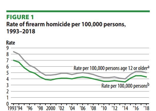 Figure 1: US Department of Justice to Homicide Rate
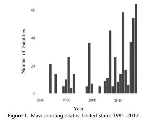
Figure 2: AAST 2018 PODIUM PAPER to Mass Shooting Deaths
Figure 1: US Department of Justice to Homicide Rate
Figure 2: AAST 2018 PODIUM PAPER to Mass Shooting Deaths
47
Figure 2 in the report illustrates this trend. Despite fluctuations in the number of such incidents, the overall trend is unmistakably upward, with a sharp upswing observed in the mid2000s.
The report acknowledges the lack of a universally accepted definition of "mass shooting," with some sources setting the bar at four or more individuals killed or injured, while others adopt a more stringent criterion. Regardless of the definition employed, the data evinces a clear trend toward increased frequency and severity of mass shootings.
The root causes of this trend are intricate and multifaceted, involving factors such as firearm accessibility, mental health, and societal dynamics. The report refutes the assertion that mass shootings are predominantly the result of mental illness and instead posits that it is the ease with which firearms, particularly high-capacity assault weapons, can be obtained that is most closely associated with these incidents.
The report further notes that most mass shooters are white men, although this demographic group is not overrepresented in the general population. This suggests that broader cultural and societal factors may contribute to the prevalence of mass shootings.
In conclusion, the rising fatality rate of mass shootings in the United States is a pressing concern and emphasizes the imperative for decisive action to address this public health crisis.
Effective strategies may encompass a spectrum of measures, ranging from stricter gun control regulations to tackling the underlying societal issues that fuel these events.
3.0 LITERATURE REVIEW
American gun deaths exceed 30,000 each year. Sex, race, and age are three characteristics that have been linked to firearm-related deaths and have been extensively researched. This literature review will provide an overview of the empirical research on firearmrelated deaths in the United States based on sex, race, and age.
The literature suggests that there are significant disparities in firearm-related deaths based on demographic characteristics. Firearm-related injuries cause more deaths among men than among women. According to a study by Anglemyer et al. From 2003 to 2012, 87% of deaths in the United States were caused by firearms. The same study also found that the firearm-related homicide rate was 6.8 times higher among men than among women.
48
There are also significant racial disparities in firearm-related deaths. The CDC estimated that African Americans died from firearm-related crimes 10 times more frequently than white non-Hispanics in 2021. Ahmad et al. Other minority groups, such as Native Americans and Hispanics, also have higher rates of firearm-related deaths than non-Hispanic whites (CDC, 2021).
Age is another demographic characteristic that is associated with firearm-related deaths. The Grinshteyn and Hemenway (2016) study found that individuals aged 15-34 die more frequently from firearm-related injuries. During 2014, firearm-related homicides disproportionately occurred among young adults. In addition, older adults are more likely to die from firearm-related suicides (CDC, 2021).
Several factors have been identified as contributing to firearm-related deaths. One of the most significant is firearm availability. 's study. Among states with higher firearm ownership rates, homicide, and suicide rates were higher. A firearm's type is also important. According to a study by Kivisto and Phalen (2018), states with more permissive laws regarding assault weapons have higher rates of mass shootings.
Other factors that have been associated with firearm-related deaths include mental illness and substance abuse. However, the research on these factors is mixed, with some studies suggesting a strong association and others finding little to no association (Swanson et al., 2015).
In conclusion, the empirical research suggests that demographic characteristics such as sex, race, and age are significant predictors of firearm-related deaths in the United States. Those aged thirty and under, African Americans, and men are particularly at risk. Availability and type of use of firearms also factor into firearm-related deaths. Therefore, evidence-based interventions are needed to address firearm-related deaths and public health crises.
4.0 DATA AND EMPIRICAL METHODOLOGY
4.1 Data
The study uses statistical data on firearm-related deaths in the United States. United States firearm-related deaths are analyzed using statistical data. National Centers for Health Statistics (NCHS) and the CDC provided reliable data sources. The data used in the study date
49
from 1999 to 2020. This data came from WISQARSTM (Web-based Injury Statistics Query and Reporting System), an official source for firearm-related deaths in the USA.
4.2 Empirical Model
Following this study by DiMaggio et al. (2018) which models the relationship between mass shooting deaths and federal assault weapons bans between 1999-2018, we have adapted and modified it to follow a newer model including age, race, and sex.
The original model is as follows:
The new model could be written as follow:
This study aims to investigate the direct effect of age, sex, race, and time on firearmrelated deaths in the US. The endogenous variable Y in equation (2) represents the number of firearm-related deaths, while the exogenous variables are age, sex, and race. To test the hypothesis, we respecify the equation as equation (3). The data for this study is obtained from the Centers for Disease Control (CDC) for the period between 1999 and 2020. The definition of firearm-related deaths in this study is consistent with the CDC's definition. Similar studies have relied on similar definitions of firearm-related deaths, such as the study by Kalesan et al. (2016) and Webster et al. (2013). Furthermore, we also analyze the effect of time (year) on firearmrelated deaths to examine whether there have been any changes over time.
The independent variables used in this study were age, sex, race, and year. Data for these variables were obtained from the Web-based Injury Statistics Query and Reporting System (WISQARS 2023), which provides information on firearm-related deaths in the US. Age was
Y = ����0 + ����1X + ����
Y (Firearm-related deaths) = ����0 (age) + ����1 (sex) + ����2 (race)+ ����3 (time in years) + ����
50
included as a variable since it is widely known that the risk of firearm-related deaths varies by age group. Similarly, sex was included since firearm-related deaths are more common among males than females. Race was also included as a variable since there are significant differences in the rates of firearm-related deaths across different racial groups. Finally, a year was included to examine if the rate of firearm-related deaths has changed over time. The dependent variable used in this study was the crude rate of firearm-related deaths per 100,000 people, which was also obtained from WISQARS 2023.
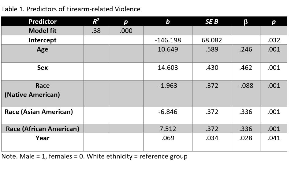
5.0 EMPIRICAL RESULTS
The empirical estimation results are presented in Table 2. The empirical estimation shows a positive relationship between age, race, and sex and the number of firearm-related deaths per 100,000 people.
51
Table 2: Regression results for the Firearm-Related Deaths
Along with these regression results are line graphs created through Excel showing the independent relationship between each of the variables associated with time in years.
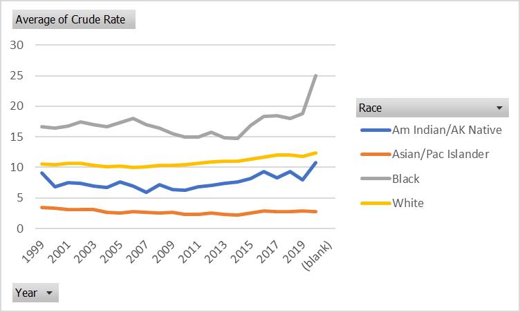
52
Figure 3. Firearm-Related Deaths Per 100,000 people based on Race.
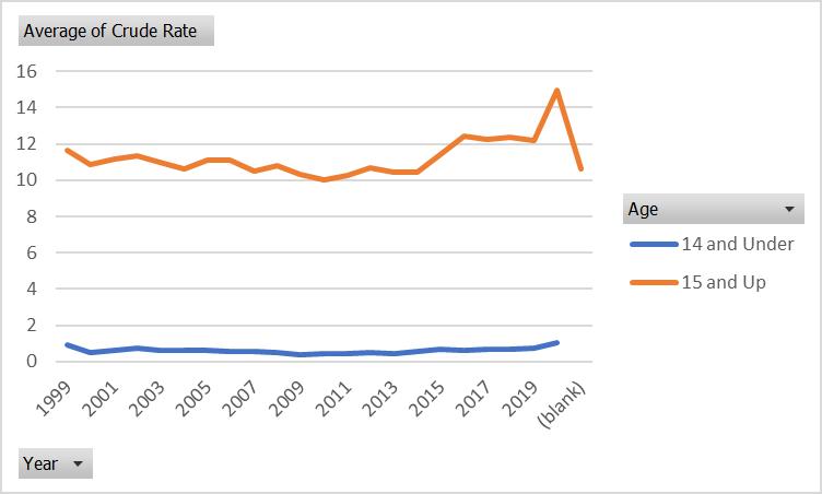
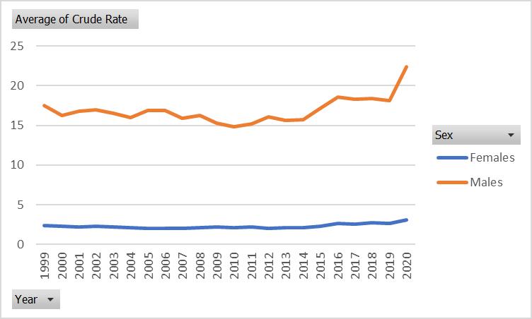 Figure 4. Firearm-Related Deaths Per 100,000 people based on Age.
53
Figure 5. Firearm-Related Deaths Per 100,000 people based on Sex.
We found that in the US, firearm-related crimes are significantly predicted by age. Increasingly, older individuals commit such crimes. In times of economic recession, firearmrelated deaths increased dramatically. Specifically, the years 2008 and the end of 2019 were marked by a notable uptick in gun violence, which we attribute to economic factors such as job loss, financial strain, and increased stress.
Furthermore, we found that African Americans are disproportionately affected by gun violence, as they are the group with the highest correlation to these crimes. Poverty and unemployment may contribute to this, causing African American communities to feel more desperate and to commit crimes more often. The US can reduce gun violence by addressing economic inequality and investing in social and economic stability.
5.0 CONCLUSION
In conclusion, regarding sex, race, and age, this empirical paper sheds light on firearmrelated deaths in the United States. Gun violence affects both men and African Americans disproportionately, according to the findings. In a study, suicide leads the list of firearm-related deaths in young adults between 18 and 34, followed by homicides and unintentional shootings. Several researchers have found that firearm violence in the United States needs policymakers' and public health officials' attention.
By addressing socioeconomic disparities and reducing firearm availability, researchers suggest reducing firearm-related deaths among vulnerable groups in the US. Utilizing a dynamic panel data model, the study examines how firearm-related deaths are interconnected across sex, race, and age. Developing evidence-based policies targeting specific populations' needs will be enabled by this study.
54
Appendix A: Variable Description and Data Source
Acronym Description Data source
CDC Government regulation information for statistics and data
Centers of Disease Control
WISQARS Data sets compiled by state reporting information to gather deaths Web Based Injury Statistics and Query Reporting System
Appendix B- Variables and Expected Signs
Acronym Variable Description What it captures Expected sign.
Crude Rate Firearm-related deaths per 100,000 people How many people have died per 100,000 firearm-related deaths.
+ Age Age of individuals Age of individuals that were surveyed between 15-85 NA Race Race of Individuals Race of individuals ranging from white, black, Asian, American Indian NA Sex Sex of individuals Biological Sex of individuals ranging from male to female NA Time Time in which the data was collected Year that the data occurred ranging from 1999-2020 NA
55
Works Cited
Ahmad, F. B., Anderson, R. N., & Farley, M. M. (2018). Deaths: Leading Causes for 2016. National Vital Statistics Reports, 67(6), 1-77.
Anglemyer, A., Horvath, T., & Rutherford, G. (2016). The accessibility of firearms and risk for suicide and homicide victimization among household members: A systematic review and metaanalysis. Annals of Internal Medicine, 165(11), 746-754.
Centers for Disease Control and Prevention. (2021). Web-based Injury Statistics Query and Reporting System (WISQARS). Retrieved from https://www.cdc.gov/injury/wisqars/index.html
Grinshteyn, E., & Hemenway, D. (2016). Violent death rates: The US compared with other highincome OECD countries, 2010. The American Journal of Medicine, 129(3), 266-273.
Kivisto, A. J., & Phalen, P. L. (2018). Effects of risk-based firearm seizure laws in Connecticut and Indiana on suicide rates, 1981 to 2015. Psychiatric Services, 69(8), 855-862.
Siegel, M., Ross, C. S., & King, C. (2014). The relationship between gun ownership and firearm homicide rates in the United States, 1981-2010. American Journal of Public Health, 104(5), 875883.
Swanson, J. W., Norko, M. A., Lin, H. J., Alanis-Hirsch, K., Frisman, L. K., Baranoski, M. V., & Easter, M. M. (2015). Implementation and effectiveness of Connecticut's risk-based gun removal law: Does it prevent suicides? Law and Contemporary Problems, 78(1), 49-74.
56
Educations Effect on Income Inequality: A Panel Data Analysis
Nicholas Garbarino
Abstract:
This paper investigates the effects of education amongst other factors on income inequality in Europe. This study examines if countries who have higher educational attainment have lower income inequality or if having higher educational attainment has no effect on income inequality.
The study will include data from several European countries over two different time periods and the results will then be compared at a country level and at an overall level to see how education affects income inequality. The regression results show that a country that has higher educational attainment is more likely to have lower income inequality. These findings are in line with most past research.
JEL Classification: I24, I25, J24
Keywords: Income Inequality, Education
Department of Economics, Bryant University, 1150 Douglas Pike, Smithfield, RI02917. Email: ngarbarino1@bryant.edu
57
1.0 INTRODUCTION
Education plays a key role in many different aspects of society. Some of the benefits of having a higher educated population include economic growth, reduced poverty, social and cultural, increased innovation and creativity and improved health and wellbeing. All these will profoundly impact the wellbeing of the country as well as the people within the country. Throughout this paper we will explore how educational attainment affects some of the countries for which are in the European Union. This study will specifically investigate how educational attainment among other factors affects income inequality.
This study is significant because of the fact that the issue of income inequality is seemingly becoming worse and worse. Now there are surely many reasons to explain why income inequality is so large and continually growing, I believe that educational attainment plays a very large role in income inequality. Because if a person is unable to get a college degree, then that will limit this person’s options to work and achieve a higher wage. It then makes it more difficult for that person to be able to pay for their children’s college tuition so that they may be able to receive a higher wage. Not only that but college tuition is rising more rapidly than any other commodity as seen in Figure 1. Every year tuition is rising which is making it more and more difficult for the average student to be able to receive a college education.
Looking into high school educational attainment is also important. In Europe it has been reported that around 85% of people age 20-24 have completed upper secondary education in 2021. While a high school or upper secondary education is good it does not necessarily provide one with some important skills and necessary tools to be truly successful. So when people are unable to go to college or any other higher educational institution they are less likely to make more money and less than half the population aged 25-34 had completed college and received a bachelor’s degree.
The main questions that are driving this research are: How can higher educational attainment influence a society and lower the income inequality gap; Second, how can education be made more available to the general public which in tail should help limit the income inequality gap; Finally, what can low income families do to break out of poverty and achieve higher wages.
58
The rest of the paper is as follows: Section 2 is a trend related to the study. Section 3 is a literature review. Section 4.1 data and estimation methodology. Section 4.2 outlines the empirical model and its variables. Section 5 presents and discusses the empirical findings based on the model. Section 6 presentS policy recommendations and research limitations. Finally, section 7 is the conclusions that have been made.
2.0 INFLATION OF TUITION AND INCOME INEQUALITY GAP
College tuition is one of the fastest rising commodities that there is. Every year college tuition at universities around the world rises and its rises at an alarming rate. The average tuition in 1963 for a four-year college education was $243.34 per year, and if you were to adjust for inflation that would me that a four-year college education should be around $2,348.67 per year according to Hanson (2022). But in reality students are having to pay on average around $40,000 annually for private institutions and around $10,000 annually for public in state institutions in America. Comparing what it was expected to be by adjusting for inflation to what tuition actually cost is very alarming to say the least. Since 1963 with adjusting for currency inflation, tuition has risen 747.8%. Something for which I found interesting is that over these past 5 years two-year institutions have seen larger increases in tuition than four-year institutions have which is evident from Figure 1. In some cases it is only a small gap but in the years 2016-17 and 2020-21 the gap equated to more than a 3%. While every case maybe be different there are some theories that have been developed to explain why college tuition has risen so rapidly. The first one being the Bennett Hypothesis, which states that the more aid that a student receives the more they are willing to pay. The second being the golden ticket fallacy, which states that the promise of a college education will result in improved future earnings, leads individuals to not look into college expenses as much. The last one that I will talk about is the Excessive Regulation theory, which states that because of the mass amounts of regulations, accreditations and federal subsidiaries it makes it difficult for innovative providers of higher education to provide and offer competition to existing universities which allows them to have higher control over price. Again every situation is different and these are not the only reasons to explain why college tuition rises so rapidly.
59
Source: National Center for Education Statistics
The second trend for which we will look at is the growing gap in income inequality. In Figure 2 you can see that around 1980 is when this gap started to expand and since this point the gap has continued to grow year after year. In regards to wealth the top 10% own around 80% of the wealth in the U.S. while the top 1% own half of that wealth. These statistics indicate how unevenly the wealth in the U.S. is spread. Looking into historical trends you can see that from the 1940s to the 1970s all income groups grow at around the same rate showing that there is less income inequality present back then. While all income groups are seemingly growing the top 5% is growing at a faster rate and endless something changes then the gap will continue to grow.
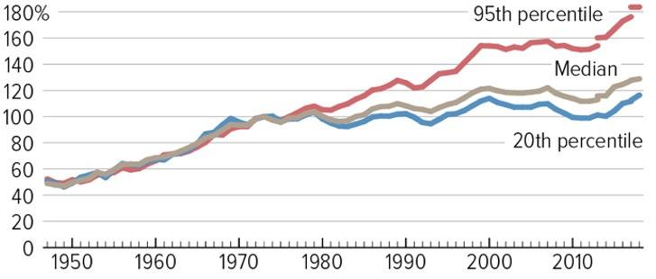
Source: CBPP calculations based on U.S. Census Bureau Data
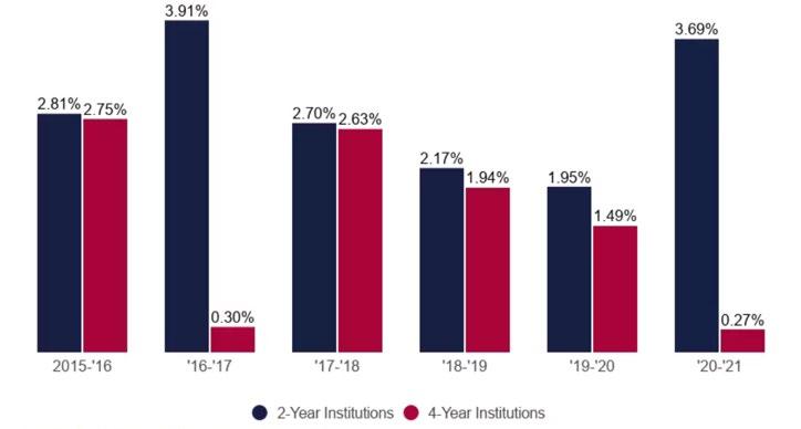 Figure 1: Annual Tuition Inflation
Figure 2: Family Income Gap
Figure 1: Annual Tuition Inflation
Figure 2: Family Income Gap
3.0 LITERATURE REVIEW 60
Education plays a large role in society and its development. There have been many different papers that discuss the role of education in societies. In the case of this research there are also a number of papers that discuss how educational attainment effects income inequality in various countries. When deciding on which papers I would include in my research I thought it was important to look at how various studies examined the effect of education on income inequality. So, I looked into studies that used poverty, migration, entrepreneurship and educational policy along with education attainment and income inequality. In a study done by Joshua Dennis Hall (2018) conclusions were made that generally when country has greater quality and quantity of education there is less income inequality. Similarly, to the study conducted by Hall (2018) a study conducted by Checchi and Werfhorst (2014) also concluded that countries that have better quality and higher quantity of education with result in lower earning gaps within their countries. When looking into developing countries the evidence is even stronger and shows a larger correlation amongst education attainment and quality of educational systems with income inequality. Education does not necessarily tell the whole story though as it is important to include other factors that are related to education or may have an impact on education. (Hall, 2018)
Educational policy can also have a large impact on income inequality. In a study done by Keller (2010), she looks into how and what type of educational policy will have an impact on income inequality. Keller (2010) concluded that countries that had higher expenditures on education would see less income inequality, specifically with developing countries. This conclusion is very logical and makes a good amount of sense. When more money is put into any resource one would expect to see better results because of it. Based on findings of all the papers that I have examined in this paper all conclude that higher educational attainment will result in lower income inequality so when countries invest in education it makes good sense that educational attainment would go up thus lowering income inequality. The study conducted by Checchi and Werfhorst (2014) also found that educational attainment is responsive to educational reform, indicating that when governments put resources into education the results will show higher educational attainment. Another study conducted by Gregorio and Lee (2002) also found that government expenditure on education as well as of general expenditures on public resources will result in lower income inequality. This was a secondary finding for Gregorio and Lee (2002) as their main finding was that education does have a negative and
61
significant effect on the GINI index. Which is in line with all other research. They also wanted to find out in what ways education effects income inequality, and they concluded that education has a significant impact on the labor market, including increasing the supply of skilled labor and reducing the wage premium for skilled workers.
One paper that I found very interesting was written by Fisher et al. (2007), and they were investigating the role of migration on education and poverty. The authors wanted to see how individuals migrating from rural areas to urban areas affected poverty in those rural areas and how education influences both poverty and migration. Controlling for the fact that bettereducated rural adults are more likely to move to urban areas, the study finds that migration has an influence on the likelihood of being poor (Fisher et al. 2007). A study by Balan et al. (2016) investigates how entrepreneurship affects educational attainment. The authors found that per capita GDP does Granger-cause both the level of educational attainment and total entrepreneurial activities of total population.
Throughout researching all these various papers all the authors concluded very similar results yet by conducting different studies. The authors used a wide range of variables to see how education affects income inequality, yet they all found that generally speaking when countries have higher educational attainment and better educational systems income inequality is lower compared to countries that have lower educational attainment. I think it’s also important to note that the effects of education were very significant when it came to developing countries. Many studies also found that when governments spend more on education, this will result in better educated individuals and lower income inequality. All of these findings are in congruence with the hypothesis that I came up with before conducting this research.
4.0 DATA AND EMPIRICAL METHODOLOGY
4.1 Data
The data utilized in this study is an annual panel data set from 2010-2020. Much of the data that was gathered was from the World Development Indicators provided by the world bank. Other resources of data include the World Governance Indicators and OECD data. Data regarding control on corruption was from the World Governance Indicators and data about educational expenditures came from the OECD dataset. The study investigates 10 countries for
62
which are a part of the EU: Spain, Italy, Malta, Sweden, Netherlands, Portugal, Lithuania, Latvia, France, Cyprus and Austria. When deciding which countries to include in the study I decided to pick countries with various levels of educational attainment based on 2019 data so that I was not looking at countries that all had high educational attainment.
4.2 Empirical Model
Applying much of the model constructed by Hall (2018) to this study, whilst drawing influence from all studies that were investigated for this paper. The model for which I came up with is:
=
GINI represents the GINI index, which measures income inequality for any given country. The GINI coefficient is a number from the range of 0 to 1, 1 representing perfect income inequality and 0 representing perfect income equality. So, the lower that the GINI coefficient if for a given country to more equally the wealth is spread out amongst its population. The Gini index is calculated by plotting the cumulative percentage of the population on the horizontal axis and the cumulative percentage of income or wealth on the vertical axis, and then calculating the area between the line of perfect equality (where the cumulative percentage of the population and income/wealth are equal) and the actual curve. GINI will represent the dependent variable for this study. When running the regression for this study the GINI variable is represented using natural log, similarly to how Hall (2018) used the GINI coefficient in his study.
I have included 5 independent variables within the empirical model. The first independent variable is GDP which represents GDP per capita of the countries involved. The second independent variable is edu which represents post-secondary educational attainment. My decision to choose post-secondary educational attainment rather than secondary educational attainment was influenced by the study conducted by Fisher et al. (2007) which was investigating the effect of educational attainment (at the post-secondary level) on migration and poverty. Fisher et al. (2007) opened my eyes up to the idea that I should be looking at the best source of education available because typically that is how your get the highest paying jobs so it should give me a good idea of how education can truly affect income inequality. Now if I were
GINI
β0 + β1GDP + β2 edu + β3 edu_exp + β4 corrup + β5trade_export + ε
63
to conduct this study again, I believe that it would be interesting to investigate educational attainment at all levels and run separate regressions for all of them. I think solid results would be uncovered in that case. The third independent variable utilized in this study is edu_exp which represents the amount of money spent per student on post-secondary education. I drew influence from 3 of the paper for which are included in my literature review which are Checchi and Werfhorst (2014), Keller (2010) and Gregorio and Lee (2002), which concluded that higher educational expenditures lead higher educational attainment and lower income inequality. Because of these findings I thought it was important to include them in my study. The fourth independent variable included is corrup which is the measurement of control of corruption. Hall (2018) included this in his model, and I believe that it is obvious that countries with lower corruption will result in less income inequality. The final independent variable for which I included in my model is trade_export which represents the high technological exports of a given country. This variable is important because to have high tech exports you need skilled laborers and to do that you need a solid educational system.
5.0 EMPIRICAL RESULTS
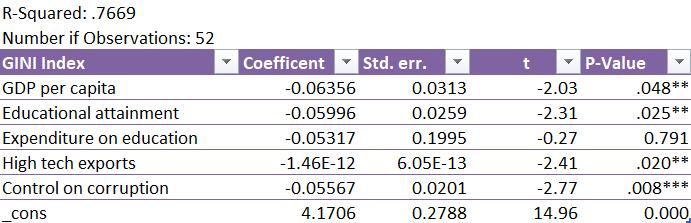
The empirical results are represented by Figure 3. I ran a simple OLS regression to see what the impact of all my dependent variables specifically, the edu dependent variable would have on the independent variable GINI. When running the regression, it is important to note that I used the natural log for the variables GINI, GDP and edu.
Note: ***, **, and * denotes significance at the 1%, 5%, and 10% respectively
Figure 3: Regression Results
64
The first thing to note is that the regression results showed that there are 4 significant independent variables present in this model. There are three variables that are significant at 5% which are GDP per capita, educational attainment and high-tech exports. Then there is also one variable for which is significant at the 1% level which is control on corruption. The one variable that is considered insignificant in this study is the expenditure on education. All these findings were expected except for the non-significance of the expenditure on education variable. As seen from past research it is significant, now the one reason that I have for it being insignificant is that the data was not entirely present and so that certainly may have played a role in it being insignificant. But in regard to all the significant variables these findings were more or less hypothesized and expected. Another notable finding from these regression results is that they are negatively correlated with the GINI index variable, and this is also expected as the lower the GINI index is the more equal income distribution is. So, if all the independent variables increase, we would see a decrease in the GINI coefficient but an increase in income equality.
Now looking at Figure 4 we can see the average GINI coefficient for the 10 countries involved in this study over the past 10 years. Then looking into Figure 5 we can see the average educational attainment for each country involved in this study over the past 10 years. My reasoning for creating these graphs was because I wanted to see how true my regression results are and by doing this, we get a good look into how the raw data that I collected compares to those results. The most significant results found from looking at these graphs is seeing that Lithuania had the highest level of educational attainment, yet they have the highest GINI coefficient, which shows that they have the highest level of income inequality. The other countries with the highest GINI coefficient are Spain, Italy, Portugal, and Lativa. For Spain, Italy, and Portugal these findings make sense and are inline with my regression results because these three countries represent the lowest levels of educational attainment in the study, but Latvia is the country with the second highest educational attainment behind Lithuania. So, these results are certainly confusing yet make sense at the same time. I believe that this shows that there are a lot of variables that affect income inequality and not one variable is responsible for a country’s income inequality.
65
Figure 4: Average GINI Coefficient
Source: Author Calculations Based on Data Provided by the World Bank
Figure 5: Average Educational Attainment
Source: Authors Calculations Based on Data Provided by the World Bank
6.0 LIMITATIONS
AND POLICY RECOMMENDATIONS
Regarding policy recommendations there are many things that can be down but this paper will just go over a few of them. The first is that countries should do their best to lower education
35.43 35.14 30.49 35.07 33.32 32.61 35.83 35.03 28.7 28.21 0 5 10 15 20 25 30 35 40 ESP ITA AUT PRT CYP FRA LTU LVA SWE NLD Average GINI Index ESP ITA AUT PRT CYP FRA LTU LVA SWE NLD 29.00% 13.71% 27.43% 18.12% 36.63% 28.28% 51.86% 40.39% 36.64% 32.22% 0.00% 10.00% 20.00% 30.00% 40.00% 50.00% 60.00% ESP ITA AUT PRT CYP FRA LTU LVA SWE NLD ESP ITA AUT PRT CYP FRA LTU LVA SWE NLD 66
costs. By doing this in theory education should be more readily available to more of the population. One risk in doing this is that the quality of the education may decrease. The second recommendation would be to invest more in schools and ensure that the schools are using the best technology and teaching the most relative information to their students. This would increase the overall quality of education being provided and result in individuals getting higher paying jobs. The last recommendation that I will give would be to increase and improve alternatives to education. As it is evident that education is not the only variable that impacts income inequality and having strong alternatives that may be cheaper than going to a post-secondary school can be very beneficial. Developing trade schools could be very beneficial as a lot of money can be made from jobs that can be obtained by going to a trade school.
Regarding the limitations of this research, I believe that I could have had a larger sample and larger spread of countries being analyzed. I only focused on countries that are a part of the EU, because I saw an interesting trend of EU countries income inequality decreasing over the past 10 years. But to be able to draw conclusions on several different areas of the world would be very interesting and would likely produce some interesting results. Another limitation here is that I only investigated post-secondary educational attainment and didn’t look into lower-level educational attainment. If I were to investigate all levels, I could draw conclusions about which level is most beneficial and lower income inequality the most. The last limitation that I will discuss is that I only investigated the quantity of education and not the quality of education.
7.0 CONCLUSIONS
In summary, I concluded that educational attainment does in fact have an effect of income inequality, along with control of corruption, high-tech exports, and GDP. Control on corruption is the most significant result of the regression which I was not anticipating but makes sense and I believe that control on corruption would be significant and effect many economic variables as it is very important to keep corruption low for countries especially those that are developing. Whilst this paper found expenditures on education to be insignificant, I do still believe that is can positively impact both educational attainment and income inequality, which is evident by the three papers done by Checchi and Werfhorst (2014), Keller (2010) and Gregorio and Lee (2002). While it is important for countries to work towards increasing educational attainment, it is certainly not the only variable that affects income inequality and, in some cases,
67
it does not have as large of an affect as one would expect. Which is evident in both Lithuania and Latvia’s case. If I were to conduct this study again there are two things for which I would want to do. The first being to look at the various levels of education and run separate regressions for each level, and the second would be to investigate the quality of education as I believe this will tell an interesting story.
68
Appendix A: Variable Description and Data Source
Acronym Description
GINI Measures income inequality for a given country
GDP Measures gross domestic products produced per capita
Edu Measures post-secondary school educational attainment (%)
edu_exp Measures the total expenditures on education per student of said nation
trade_export Measures the total amount in dollars of a country’s high technological exports
corrup Measures the level of control on corruption a country has
Data Source
World Development Indicators
World Development Indicators
World Development Indicators
OECD Database
World Development Indicators
World Governance Indicators
69
BIBLIOGRAPHY
Balan, F ., Ozekicioglu, S & Kilic, C, (2016). "Determining the causal relationships among entrepreneurship, educational attainment and per capita GDP in high-income OECD countries," Theoretical and Applied Economics, Asociatia Generala a Economistilor din Romania - AGER, vol. 0(3(608), A), pages 243-256, Autumn.
Weber, B., Marre, A., Fisher, M., Gibbs, R., & Cromartie, J. (2007). Education’s Effect on Poverty: The Role of Migration. Review of Agricultural Economics, 29(3), 437–445. http://www.jstor.org/stable/4624853
Gregorio, J & Lee, J, (2002). "Education and Income Inequality: New Evidence From Cross‐Country Data," Review of Income and Wealth, International Association for Research in Income and Wealth, vol. 48(3), pages 395-416, September.
Hall, J, (2018). "The effects of the quality and quantity of education on income inequality," Economics Bulletin, AccessEcon, vol. 38(4), pages 2476-2489.
Hanson, M. (2022). College tuition inflation [2023]: Rateincreasestatistics.Education Data Initiative. Retrieved March 27, 2023, from https://educationdata.org/college-tuitioninflation-rate
Keller, K. R. I. (2010). How Can Education Policy Improve Income Distribution? An Empirical Analysis of Education Stages and Measures on Income Inequality. The Journal of Developing Areas, 43(2), 51–77. http://www.jstor.org/stable/40376250
70
An Empirical Analysis of the Impact of Unemployment Rate and Economic Development Level on Income Inequality
Wenyi Gua
Abstract:
This study used linear regression analysis to inspect influence of unemployment rates and economic development levels on income inequality in the United States and Germany. The results indicate that the level of economic development is the main driving factor for inequality of income in America, while in Germany, high unemployment and inflation can exacerbate income inequality. This study emphasizes the importance of labor market policies, social welfare policies, and tax policies in reducing income inequality. While the analysis only covers two countries, the results have significant policy implications for addressing income inequality. Future research can expand on the factors that contribute to income inequality.
JEL Classification: A1, C1, C5, J3, J6
Keywords: FDI, Income inequality, CPI, GDP per Capital, Unemployment rate
a Undergraduate Student, Bryant University, 1150 Douglas Pike, Smithfield, RI 02917.
Phone: (401) 757-9565. Email: wenyiwinnie.gu@outlook.com.
71
1.0 INTRODUCTION
Income inequality has always been a long-standing problem in many countries around the world. In recent years, this issue has attracted attention due to its adverse effects on economic growth, social stability, and poverty reduction. Although the factors contributing to income inequality are complex and multifaceted, this study focuses on the impact of unemployment rates and economic development levels in America and Germany on income unfairness. In addition, this study analyzed how foreign direct investment and consumer price indices affect income inequality in these two countries. The United States and Germany are two prominent economies with vastly different economic systems, but both countries are struggling with income inequality. Similarly, in Germany, although the country is famous for its strong welfare state, income inequality has been increasing since the beginning of the 21st century.
The purpose of this research is to improve our comprehend and understanding of the driving factors of income unfairness in America and Germany. From the perspective of national governments, this study is important and meaningful as income inequality can affect economic growth, social welfare, and political stability. By identifying the key determinants of income inequality, policymakers can develop effective policies to address this issue. The relevance of this study lies in increasing literature on the effect of unemployment rate and economic development level on income unfairness, while also considering foreign direct investment and consumer price index as potential drivers of income inequality. Previous studies either focused solely on unemployment or economic development or did not explore the role of foreign direct investment and consumer price indices in shaping income inequality. This study provides a comprehensive analysis that considers all four factors simultaneously, which is crucial for policymakers seeking to design effective policies to reduce income inequality.
This paper is guided by three research objectives: firstly, using relevant economic data from the United States and Germany, to study the connection between economic development level, unemployment rate, and income unfairness; Secondly, study the role of foreign direct investment and consumer price indices in causing income inequality in these two countries; Thirdly, analyze the potential interaction between these factors and income inequality. To achieve these goals, this study uses the Gini coefficient as the dependent variable, and unemployment rate, per capita GDP, CPI, and FDI as independent variables. The main part of this paper is organized as follows:
72
2.0 shows the trend of changes in the Gini coefficient in Germany and the United States. 3.0 presents a literature review of the references used in the research paper. 4.0 discusses data and regression analysis methods. Finally, 5.0 introduces and discusses the empirical analysis results.
6.0 Draw conclusions.
2.0 Trend
Figure 1 shows the trend changes in Gini coefficient in Germany from 1991 to 2018. In economics, the Gini index is a statistical discrete measure aimed at representing income inequality, wealth inequality, or consumption inequality. In this chart, the closer the Gini index is to 0, the more equal it is, while the closer the index is to 100, the more unequal it is. From this graph, it can be seen that the German Gini coefficient presents a fluctuating upward trend.
Source:
Figure 2 shows the change trend of the Gini coefficient in United States from 1991 to 2018. From this graph, it can be seen that the United States Gini coefficient presents a fluctuating upward trend.
Figure1: Variation Diagram of Gini Coefficient in Germany
FRED Economic Data
26.0 27.0 28.0 29.0 30.0 31.0 32.0 33.0 Germany GINI 73
Figure2: Variation Diagram of Gini Coefficient in United States
Source: FRED Economic Data
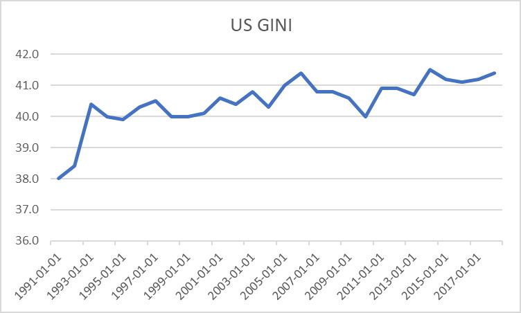
3.0 LITERATURE REVIEW
Not only in the America and Germany, but also in other countries, income inequality is a major issue. The study investigated the factors that contribute to income inequality. This literature review examines previous research findings on factors affecting income unfairness in America and Germany. The paper by Autor and Dorn (2013) found that the key factors leading to inequality of income in America are the increase of less-technical ability service industry works and the unequal supply of the America manpower market. Heimberger (2018) conducted a crossborder analysis and found that employment has a remarkable influence on income unfairness. The paper suggests that countries with higher employment rates are accompanied by lower levels of income unfairness, which is higher in countries with lower employment rates. Meanwhile, Rehm and Biewen (2014) argue that the connection between unemployment rate and income inequality in Germany changed in the early 21st century. They found that unemployment is no longer an important predictor of income inequality in Germany. This discovery is not only found by Rehm and Biewen, but also by Schmid and Modrack (2014), which found that this relationship weakened in the early 21st century. The study attributed the change to policies aimed at increasing the flexibility of the German labor market.
74
Burkhauser, Larrimore, and Simon's (2012) paper showcases the economic fitness of the American bourgeoisie, and they found that although this class did not decline, it did not experience substantial growth. The OECD (2011) released a report on the intensification of income inequality, which found that in the past few decades, income inequality has risen in most OECD countries, with the America having the highest level of income inequality. Meanwhile, Saez (2017) studied income unfairness in America and found that income inequality is at its highest level since the 1920s. In addition, research has found that between 2009 and 2015, the highest 1% of people accounted for 52% of the total income growth in the US, which is a typical manifestation of income inequality. Economic development level has also been found to be a significant factor in income inequality. Kaldor (1957) proposed that economic growth would lead to a reduction in income inequality, because economic growth will increase the demand for labor, leading to an increase in worker wages.
However, subsequent research results were mixed. Dollar and Kraay (2002) used 40 years of data from 63 countries and found that economic growth has a slight adverse effect on income unfairness, but this effect is not statistically remarkable. Meanwhile, Alesina and Rodrik (1994) found no clear relationship between income unfairness and economic growth in a sample of 16 developed countries. More recent researches have focused on the impact of globalization on income unfairness. Milanovic (2016) argued that globalization has contributed to the rise of income inequality by creating winners and losers in the global economy. The winners tend to be highly skilled workers in developed countries, while the losers tend to be low-skilled workers in developing countries. Milanovic also found that the indirect impact of globalization has led to a decrease in the proportion of labor income to GDP, further exacerbating income inequality. Similarly, Stiglitz (2012) argued that globalization has contributed to the rise of income inequality by allowing capital to flow freely across borders, while labor remains constrained by national borders. This has led to a situation where capital owners can extract more value from workers, while workers are unable to negotiate better wages and working conditions. Stiglitz also pointed out that the impact of globalization will also lead to a decrease in the power of trade unions, further weakening the bargaining power of workers, thereby affecting their ability to compete for their legitimate rights. Other scholars have pointed out the role of technological change in leading to income unfairness. Brynjolfsson and McAfee's (2014) study suggests that technological progress leads to extreme inequality in the labor market, where highly skilled
75
workers benefit from acquiring new technologies, while low-skilled workers are easily replaced due to a lack of technology. They also pointed out that the decrease in the proportion of labor income due to technological progress has further exacerbated income inequality.
In summary, the literature review indicates that the connection between unemployment rate and income unfairness is worth studying and varies among countries. However, higher employment rates tend to lead to lower levels of income unfairness. Moreover, the review highlights the growing income inequality in many countries, particularly in the United States. Policymakers should consider implementing measures to address income inequality, such as policies aimed at increasing employment rates, progress sive taxation, and social welfare programs. The literature on the effect of unemployment rates and economic development levels on income unfairness is extensive and multifaceted. Although there is consensus that employment rates and economic growth can have a certain effect on reducing income unfairness, the relationship is complex and depends on a range of factors, including globalization, technological change, and government policies. It is evident that addressing income inequality requires comprehensive consideration, taking into account various factors, and seeking to create more equitable resource and opportunity allocation.
4.0 Data and empirical methodology
4.1DATA
The study used data from 1991 to 2018. This paper mainly uses time series for research. The data mainly comes from the Federal Reserve's economic data website. The publicly available FRED data includes data on major economic indicators in the United States and Germany. Table 1 and Table 2 provide a summary of statistical data.
Variable n min max average sd GINI 28 28.300 31.800 30.193 1.153 unemployment rate 28 3.400 11.200 7.400 2.135 76
Table 1 Describe the statistical analysis about Germany
According to the descriptive statistical analysis of sample data in Germany, the average GINI is 30.193, the average unemployment rate is 7.400, and the average CPI is 1.809. The average Foreign direct investment net inflows were 57.095 and the average GDP per capita was 36,124.968.
According to the descriptive statistical analysis of sample data in America, the average of GINI is 40.471, the average of unemployment rate is 5.933, and the average of CPI is 0.188. The average for Foreign direct investment net inflows was 219.135, while the average for GDP per capita was 49,978.277.
Variable n min max average sd CPI 28 0.315 5.075 1.809 1.142 Foreign direct investment net inflows 28 -20.410 248.010 57.095 55.074 GDP per capita 28 30615.14042928.74136124.968 3903.955
Table 1 Describe the statistical analysis about Germany
Variable n min max average sd GINI 28 38.000 41.500 40.471 0.796 unemployment rate 28 3.900 9.630 5.933 1.593 CPI 28 0.012 0.334 0.188 0.075 Foreign direct investment net inflows 28 30.310 511.430 219.135 129.923 GDP per capita 28 38739.800 59607.390 49978.277 6097.942
Table 2 Describe the statistical analysis about United States
77
4.2 EMPIRICAL MODEL
The model of this research paper is:
εβββββ +++++=443322110XXXX Y
Table3 Variable meaning and description symbol variable meaning dependent variable Y GINI a measure of income inequality within a population
Core explanatory variables X1 Unemployment Rate
The proportion of labor force who are in process of seeking job despite temporarily losing their jobs
X2 GDP per capita the total GDP of a country divided by its population control variable X3 Customer Pirce Index This is used to measure the average price at which households purchase a basket of goods and services
X4
Foreign direct investment net inflows
This represents an investment by a company from country A in a company or entity
78
from country B.
These independent variables are significant indicators of a country's economic performance and can have a substantial effect on income unfairness. The unemployment rate, for instance, may be positively correlated with income inequality since the unemployed may have little access to income and resources, while those who are employed earn relatively higher incomes. The per capita GDP is positively associated with income inequality as higher levels of wealth may translate into a higher concentration of income among the rich. CPI, on the other hand, may have a negative association with income inequality since inflation disproportionately affects those with low-income. Finally, FDI may have a positive association with income inequality since it may lead to more concentration of wealth among foreign investors, who are often wealthy.
In summary, this model seeks to explain income inequality by examining the connection between the Gini index and the independent variables of unemployment rate, per capita GDP, CPI, and FDI. By understanding these relationships, policymakers can develop strategies that may help to mitigate income inequality and promote a more equitable distribution of wealth within a society.
5.0 EMPIRICAL RESULTS
The empirical results are shown in Table 4.
Table4: Regression results for the Germany and United States Variable Germany United States constant -111.783*** (-6.214) -23.865* (-1.938) unemployment rate 0.183* (2.526) -0.112* (-1.883) GDP per capita 13.375*** (8.012) 6.065*** (5.241) 79
The values in parentheses are T values *P<0.05 **P<0.01 ***P<0.001
R 2, with values ranging from 0 to 1, indicates a higher degree of fit for the model as it approaches 1, indicating that the independent variable can explain 81% of the variation of the dependent variable.
F-test is used to test whether the independent variable has statistical significance to the regression model of the dependent variable.
Germany:
Using the data in Table 4, the Gini modulus is used as the dependent variable, with unemployment rate, per capita GDP, CPI, and net foreign direct investment as independent variables. Through linear regression analysis, it can be concluded that the formula for this model is: GINI=-111.783 + 0.183*unemployment rate + 13.375*GDP per capita + 0.265*CPI0.003*Foreign direct investment net inflows, The R square value is 0.810. It means that the unemployment rate, GDP per capita, CPI and Foreign direct investment net inflows can explain 81.0% of the change in GINI. The study found that the model passed the F-test (F=24.501, p=0.000<0.05). This indicates that at least one of the factors such as unemployment rate, per capita GDP, CPI, and net inflows of foreign direct investment will have an impact on the Gini coefficient. The final especially analysis indicates that: The regression index value of unemployment rate is 0.183(t=2.526, p=0.019<0.05), which means that unemployment rate will have a remarkable active effect on GINI. The regression index value of GDP per capita is 13.375(t=8.012, p=0.000<0.01), which means that GDP per capita will have a remarkable positive effect on GINI. The regression index value of CPI is 0.265(t=2.213, p=0.037<0.05),
CPI 0.265* (2.213) -1.074 (-0.828) Foreign direct investment net inflows -0.003 (-1.170) -0.002 (-1.464) n 28 28 R 2 0.810 0.708 Adjust R 2 0.777 0.658 F F (4,23) =24.501, p=0.000 F (4,23) =13.959, p
=0.000
80
indicating that CPI will have a remarkable positive influence on GINI. The regression index value of Foreign direct investment net inflows was -0.003(t=-1.170, p=0.254>0.05). This means that Foreign direct investment net inflows will not affect GINI. The summary analysis shows that unemployment rate, GDP per capita and CPI will have a significant positive impact on GINI. However, Foreign direct investment net inflows will not affect GINI. United States:
By analyzing the data in Table 4, with Gini coefficient as the dependent variable and unemployment rate, per capita GDP, CPI, and net foreign direct investment as independent variables, and using linear regression analysis method, the formula of the model can be obtained as follows: Gini coefficient=-23.865 0.112 * unemployment rate+6.065 * per capita GDP -1.074 * CPI-0.002 * net foreign direct investment. The R-squared value of the model is 0.708, which represents the unemployment rate, per capita GDP CPI and net inflows of foreign direct investment can explain the 70.8% change in the Gini coefficient. When F-test was conducted on the model, the data showed that the model passed the F-test (F=13.959, p=0.000<0.05). In other words, at least one of the factors such as unemployment rate, per capita GDP, CPI, and net inflows of foreign direct investment will have an impact on the Gini coefficient. The regression index value of unemployment rate is -0.112(t=-1.883, p=0.072>0.05), which means that unemployment rate will not have an impact on GINI. The regression index value of GDP per capita is 6.065(t=5.241, p=0.000<0.01), which means that GDP per capita will have a remarkable active effect on GINI. The regression index value of CPI is -1.074(t=-0.828, p=0.416>0.05), which means that CPI has no impact on GINI. The regression index value of Foreign direct investment net inflows was -0.002(t=-1.464, p=0.157>0.05). This means that Foreign direct investment net inflows will not affect GINI. The summary analysis shows that GDP per capita has a significant positive impact on GINI. However, unemployment rate, CPI and Foreign direct investment net inflows do not affect GINI.
81
Assuming a serious collinearity problem occurs, the analysis results will be instability, and the sign of the regression index will be completely inverse to the reality status. This will result in insignificant outcomes for independent variables that should be significant, while insignificant outcomes for independent variables that should not be significant. In this case, the effect of multicollinearity should be eliminated. From Table 5, it can be seen that the VIF of the independent variable is less than 10. This result can be considered that there is no multicollinearity in the independent variable.
Germany VIF United States VIF unemployment rate 2.179 1.127 GDP per capita 2.967 2.671 CPI 1.698 1.174 Foreign direct investment net inflows 1.322 2.820
Table 5 Multiple collinearity test
Germany United States constant -110.668*** (-5.971) -14.064 (-1.064) Lag1_unemployment rate 0.203** (2.696) -0.048 (-0.800) Lag1_GDP per capita 13.257*** (7.706) 5.094*** (4.067) Lag1_CPI 0.225* (1.808) 0.563 (0.474) Lag1_Foreign direct investment net inflows -0.000 (-0.086) -0.001 (-0.865) n 27 27 R 2 0.805 0.630 82
Table 6 Robust test
Purpose: To test the reliability of the regression results (whether the obtained research conclusions are stable)
In order to test the robustness of the model, first-order lag processing is carried out on the independent variables. The lag regression results show that GDP per capita has a stable positive impact on GINI. For Germany, unemployment rate has a remarkable positive effect on GINI. For the United States of America, the unemployment rate has a volatile effect on GINI. To sum up, the level of economic development has a remarkable active effect on income gap, that is, the higher the level of economic development, the income gap will increase significantly. In terms of unemployment rate, the impact of higher unemployment rate on income gap is different in the United States and Germany. In Germany, the higher unemployment rate will significantly increase the income gap, while in America, the unemployment rate has a stable influence on income gap.
6.0 CONCLUSION
This study aims to research the effect of unemployment rate and economic development level on income inequality in America and Germany. This study uses linear regression analysis to test the connection between the dependent variable (Gini index) and the independent variable (unemployment rate, GDP per capita, CPI, and FDI). Based on the results of regression analysis, the study found that in Germany, unemployment rate, per capita GDP, and CPI have an outstanding positive effect on income inequality (measured by the Gini index). In America, research has found that only per capita gross domestic product has a remarkable active influence on income inequality, while unemployment rate, CPI, and foreign direct investment net inflows did not affect income inequality significantly.
The results of this study provide important insights into the factors contributing to income inequality in Germany and the United States. Specifically, in Germany, income inequality is positively correlated with high unemployment and inflation. In contrast, in the
Adjust R 2 0.769 0.563 F F (4,22)=22.674,p=0.000 F (4,22)=9.380,p=0.000
83
United States, measured by per capita GDP, income inequality is largely driven by the level of economic development. The findings are consistent with previous research that has shown that economic development, as well as labor market policies, social welfare policies, and tax policies, are important determinants of income inequality (Bourguignon, 2015). The study has some limitations that should be considered. Firstly, the analysis only includes four independent variables, and there may be other factors that contribute to income inequality that are not included in the model. Secondly, the study is based on cross-sectional data, and causality cannot be established with certainty. Finally, as this analysis only covers the United States and Germany, its results may not be widely applicable to other countries.
In conclusion, the study provides important insights into the impact of unemployment rate and economic development level on income inequality in the United States of America and Germany. The findings suggest that economic development level is an important determinant of income inequality in the United States, while unemployment rate, per capita GDP, and CPI are important determinants of income inequality in Germany. The findings have important policy implications for addressing income inequality in these countries, including policies that promote economic growth, reduce inflation, and address labor market inequalities. Future research could explore the impact of other factors on income inequality, including tax policies, social welfare policies, and other economic and social factors.
84
BIBLIOGRAPHY
Alesina, A., & Rodrik, D. (1994). Distributive politics and economic growth. The Quarterly Journal of Economics, 109(2), 465-490.
Autor, D. H., & Dorn, D. (2013). The growth of low-skill service jobs and the polarization of the US labor market. American Economic Review, 103(5), 1553-1597.
Brynjolfsson, E., & McAfee, A. (2014). The second machine age: Work, progress, and prosperity in a time of brilliant technologies. WW Norton & Company.
Bourguignon, F. (2015). The globalisation of inequality. Princeton University Press.
Burkhauser, R. V., Larrimore, J., & Simon, K. I. (2012). A "second opinion" on the economic health of the American middle class. National Tax Journal, 65(1), 7-32.
Dollar, D., & Kraay, A. (2002). Growth is good for the poor. Journal of economic growth, 7(3), 195-225.
Heimberger, P. (2018). Employment and income inequality: A cross-country analysis. Journal of Economic Issues, 52(1), 187-204.
Kaldor, N. (1957). A model of economic growth. The Economic Journal, 67(268), 591-624.
Milanovic, B. (2016). Global inequality: A new approach for the age of globalization. Harvard University Press.
OECD (2011). Divided we stand: Why inequality keeps rising. OECD Publishing.β
Rehm, M., & Biewen, M. (2014). Unemployment and income inequality revisited: An analysis of German micro data. Journal of Economic Inequality, 12(1), 21-40.
Rehm, M., & Biewen, M. (2014). Unemployment and income inequality revisited: When flow matters. Journal of Economic Inequality, 12(1), 21-40.
Saez, E. (2017). Income and wealth inequality: Evidence and policy implications. Contemporary Economic Policy, 35(1), 7-25.
85
The Determinants of Carbon Emission in Asia and Europe: A Panel Data Analysis
Erika Hauser
Abstract:
This paper investigates the numerous variables that influence carbon emissions in selected Asian and European countries. The study examines the countries with the highest gross domestic product (GDP) in each region, considering the possible impact of economic growth on greenhouse gas emissions. The study also analyzes the role of other variables such as tourism, foreign direct investment (FDI), ecological footprint level (EFL), and agricultural output. The ecological footprint level is modeled by global hectare or the countries’ gha, which is a measure of the impact of human activities on the environment. The study estimates tourism and FDI reduce emissions, while economic growth, agriculture, and ecologic footprint level increase carbon emissions.
JEL Classification: O13, Q53
Keywords: Natural Resources, Environmental Economics, Air Pollution
86
The state of the planet has been in question for future years as greenhouse gases (GHG) are emitted into the atmosphere, the main contributor being carbon dioxide. This happens through the burning of fossil fuels, which occurs globally, as energy use for electricity, transportation, heating, and other purposes. These GHG emissions are causing the planet to warm, sea levels to rise, ice caps to melt, air pollution, and many other things. In some extreme cases, humans are being forced to migrate from their homes because they are no longer habitable
Countries have set parameters and regulations to try and reverse or lessen the damage caused by reducing their carbon emissions; however, certain industries make it difficult to operate without the negative effects. China is a leading contributor to the release of carbon dioxide and has shown a dramatic increase throughout the decades because of its staggering economic growth. This study aims to enhance understanding of the leading economic and environmental contributors to higher emissions of carbon dioxide in Asia and Europe. The countries studied have the top ten GDP in Asia and the top nine in Europe while analyzing FDI, economic growth, ecological footprint level, agriculture, and tourism. From a policy perspective, this analysis is important because it will show whether there is a linkage between wealth and carbon emissions in a country. The relevance of this study is that it can provide insight into how the emission of greenhouse gases can be reduced based on what the leading factors are that cause it.
It is important to decrease carbon emissions because greenhouse gases (GHG) lead to global warming, which will have serious effects on the environment as it continues to worsen: some examples are the sea level will rise, polar ice will be lost, and the ocean will increase in temperature. These events will lead to the extinction of species, the displacement of people in areas that are no longer suitable for living, and a decrease in biodiversity, which means less food.
Short-term studies show that efforts to reduce carbon emissions will decrease economic growth, but as countries continue to create incentives to “go green”, new industries are blooming and thriving. One sector of economic growth is measured through transportation, which is one of the highest pollutants; the promotion of biofuels
1.0 INTRODUCTION
87
and electric vehicles has been introduced to reduce the negative effects of GHG emissions through transport. (Rehermann and Pablo-Romero, 2018).
This paper was guided by three research objectives that differ from other studies: First, it investigates the ecological footprint level of each country in the study, which measures how fast humans utilize resources and generate waste compared to how fast nature can absorb the waste and generate resources. Second, it incorporates the tourism expenditures in each country which refers to the amount of money spent by tourists or visitors in a particular destination or country. Finally, this study will investigate the agricultural share of gross domestic product (GDP) as a proxy for economic growth; this will measure agriculture, fishing, and forestry.
The paper is structured as follows: Section 2 provides a concise literature review. Section 3 outlines the empirical model, while Section 4 discusses the data and estimation methodology. In Section 5, the empirical results are presented and analyzed. The paper concludes the findings in Section 6.
2.0 TEND OF CO2 EMISSIONS
Figure 1 shows that carbon dioxide emissions in Asia, measured in metric tons per capita, have been on increasing for the past three decades. The diagram depicts a rise in CO2, which is most likely due to a spike in economic growth in the region. Saudi Arabia had the highest per capita CO2 emissions in 2020, but it has since decreased. Now, Qatar, which shares a land border with Saudi Arabia, is the top country in the world with the highest emissions per capita at 37.29 tons per capita.
88
Figure 1: Carbon Emissions in Asia 1990-2020
Source: World Bank Indicators Database
Figure 2 shows the course of carbon dioxide emissions in Europe over the past thirty years, which differs from Figure 1. The graph displays there is a decrease in emissions, while in Asia it was mostly increasing. There is a much lower correlation between economic growth and CO2 emissions but showed a greater relationship between agriculture.
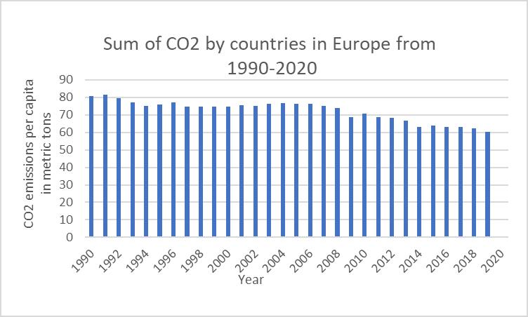
Source: World Bank Indicators Database
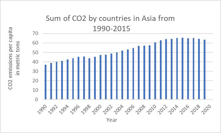 Figure 2: Carbon Emissions in Europe 1990-2020
89
Figure 3 shows the combined sum of CO2 emissions per capita in metric tons for Europe and Central Asia. In total, the overall production level decreases significantly for these regions; however, when looking at the wealthiest countries in Asia and some in Europe, the emissions increase throughout the years. This study asserts the reason for this is that the richer countries saw a spike in economic growth during this time, which led to higher emissions in those countries.
Source: World Bank Indicators Database
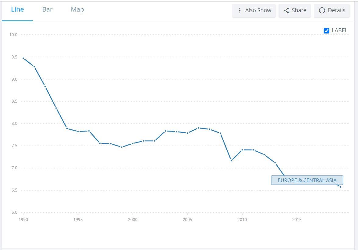
3.0 LITERATURE REVIEW
The environmental Kuznets curve (EKC) hypothesis was introduced by Grossman and Krueger (1995), which denotes to an inverted U-shaped relationship concerning environmental degradation and per capita income. Essentially, the hypothesis states that environmental quality decreases initially to then increases as per capita income rises. The study done by Fang et al. (2018) examines the EKC using trade openness to determine at which point it changes in China. The paper focuses on trade and the environment and
Figure 3:
90
measures the relationship between trade and its effect on pollution and economic growth. It has been concluded that developing countries are larger contributors to environmental pollution through economic growth, especially those that have seen rapid growth from 1990 and onwards, and the total figures of greenhouse gas emissions have more than doubled (Jahanger et al., 2022). The study conducted by Zhang and Zhang (2018) indicates that the EKC hypothesis holds true for China, and while both services trade and exchange rates had a negative effect on China's carbon emissions,
The tourism industry is a significant contributor to the global economy, accounting for a considerable portion of the world's gross domestic product (GDP) and employing a substantial percentage of the global workforce. Additionally, it plays a significant role in overall exports and foreign direct investment (FDI), making it a crucial aspect of the world's tourism investment. However, the expansion of this industry has led to a rise in fossil fuel consumption and significant greenhouse gas (GHG) emissions (Jebli et al., 2019). While Zhang and Zhang (2018) saw a negative effect on carbon emissions from services trade and exchange rates, FDI inflows had a positive impact.
The study by Dogan et al. (2022) confirms the Environmental Kuznets Curve Hypothesis for G7 countries and looks at the impact of environmental taxes on energy consumption and CO2 emissions. It's the first study to investigate the effect of an environmental tax on both renewable and non-renewable energy consumption, natural resource rent, and CO2 emissions. The results show that environmental taxes are effective in reducing emissions and that higher taxes lead to more significant effects on traditional energy consumption, natural resources rent, and renewable energy consumption.
The transportation industry uses a lot of fossil fuels and contributes significantly to greenhouse gas emissions. To reduce its impact on the environment and achieve carbon neutrality, developing smart transportation has become a popular solution. Zhao et al (2021) uses spatial econometric models to investigate the impact of smart transportation on CO2 emissions in China. The study found that smart transportation is becoming more prevalent in China, but there are differences between regions. The study also found that
91
smart transportation can have an impact on CO2 emissions, not only in the transportation industry but also in other areas. There is a spillover effect, meaning that neighboring provinces' development of smart transportation can also affect carbon mitigation in a given province. Gillingham et al. (2021) look at the effects of carbon pricing and its impact on electric cars and concluded that if carbon prices remain moderate like they are now, electric cars will probably still be charged using coal-based electricity. This was confirmed using a detailed model that looks at both transportation and electricity. However, if carbon prices increase significantly, then the situation will change and electric cars will more likely be charged using cleaner energy sources.
4.0 DATA AND EMPIRICAL METHODOLOGY
4.1 Data
The study uses annual data (panel data) from 1990 to 2020. Data were obtained from the Bureau of Economic Analysis (BEA) website, World Development Indicators, and World Population Review. Summary statistics for the data are provided in Table 1. Originally, the variables from the papers were going to include transportation, renewable energy, and trade; however, after further review, the model was simplified to only five dependent variables.
Table 1 Summary Statistics
Variable Observation Mean Std. Dev. Min Max CO2 300 5.293967 4.228137 .51 17.3 FDI 310 1.96e+10 4.69e+10 -4.95e+09 2.91e+11 Growth 308 9327.516 11884.67 302 49145 EFL 290 2.770586 1.626906 .72 6.32 Agriculture 306 11.09006 7.347499 .9966057 27.66271 Tourism 240 2.05e+07 3.42e+07 369000 1.63e+08 92
4.2 Empirical Model
Following Jebli et al. (2019) and Jahanger et al. (2022) the study adapted and modified the relationship between carbon dioxide emissions, tourism, and economic growth:
I have added FDI, economic footprint level, and agriculture.

The model could be written as follow:


is the measure of carbon dioxide emissions per capita in country i at year t

Measured in metric tons, represents how much carbon is being emitted each year throughout the regions. Carbon dioxide is a greenhouse gas that comes from the removal of and burning of fossil fuels, and has been increasingly warming the atmosphere of the earth. The definition of CO2 in this paper is consistent with the definition used in various studies, (Dogan et al. 2022; Jahanger et al. 2022; Jebli et al. 2019).
There are five independent variables obtained from various sources. Appendices A and B provide data sources, acronyms, explanations, expected signs, and justification for using the variables. First, (annual flow of FDI from the US to country at year ) represents funds that US parent companies provide to their foreign affiliates. represents the per capita GDP of each country in USD which data is obtained from the WDI is a proxy for economic growth, which measures a share of GDP per country. measures the economic footprint level of each country in global hectares, which is how fast we consume resources and generate waste compared to
(1)
93
how fast nature can absorb our waste and generate resources. Lastly, measures tourism arrivals and how many tourists visit the country each year.
5.0 EMPIRICAL RESULTS
The study's empirical findings are presented in Tables 2 and 3, demonstrating a statistically significant positive correlation between ecological footprint level and economic growth in regard to carbon dioxide emissions. Both a fixed-effect and randomeffect regression are run. Table 2 displays regression results for the Asian countries, while Table 3 showcases the results for the European countries.
Note: *** , **, and * denotes significance at the 1%, 5%, and 10% respectively. Standard errors in parentheses

CO2 OLS FE RE Constant -3.300546 (.7721003) .4732555 (1.050576) .54363 ( .8873555) FDI -2.20e-12 (9.21e-12) 1.83e-12 (7.69e-12) 1.89e-12 (7.77e-12) Growth -.0000575** (.0000239) .0000803*** (.0000109) .0000793*** (.0000111) EFL 2.942868*** (.1630489) 1.73921*** (.2496486 ) 1.762006*** (.2615809) Ag .0691275* (.0343078) -.0611998* ( .0427496) -.061319* (.0419836) T 8.67e-12 (2.18e-11) -2.75e-11 (1.38e-11) -2.83e-11 (1.38e-11) R2 0.9038 0.8617 0.8629 Number of obs. 189 189 189
Table 2: Regression results for the 10 Asian countries
CO2 94
Table 3: Regression results for the 9 European countries
In Table 2, the Growth and EFL variables are significant at the 1% level. The parameter estimate of Growth is consistent with the results of Jahanger et al. (2022) and Jebli et al. (2019), which implied that economic growth was positively associated with CO2 emissions in the Asian region, more specifically China. EFL is significant because it represents the use of natural resources, such as the burning of fossil fuels which emits carbon dioxide. The results conclude that the correlation is more statistically significant over the years which is shown within the random-effects regression. The effect of T is also significant at the 5% level; however, the analysis reveals that FDI and Ag on carbon emissions proved to be statistically insignificant. Overall, the regression suggests that economic growth and ecological footprint levels have a positive and significant relationship with CO2 emissions. However, the relationship between CO2 emissions and agriculture and tourism is not statistically significant. The R-squared values indicate that there may be substantial differences in CO2 emissions between countries that are not accounted for in this model.
OLS FE RE Constant -1.312503 (1.774682) 5.282834 (1.942821) 5.219532 (2.027002) FDI 4.57e-12** (1.93e-12) -1.33e-13 (3.54e-13) -1.05e-13 (3.53e-13) Growth -.0000214** (.0000108) -.0000187** (8.62e-06) -.0000196** (8.45e-06) EFL 1.28308*** (.2366782) .6296567 (.3667816) .6326294* (.3677761) Ag .7435829 (.1947978) .1025887 (.175187) .104029 (.1641628) T 4.11e-11 (6.01e-12) -9.22e-12 (7.12e-12) -8.10e-12 (6.86e-12) R2 0.4936 0.1458 0.1623 Number of obs. 154 154 154
95
Table 3 similarly shows more statistical significance through the years within the random-effects regression; however, it is substantially less correlated than Table 2. With R-squared values of only 0.1458 and 0.1623, the overall results are insignificant. Only the variables of Growth and CO2 are statistically significant at the 10% and 5% levels. The coefficients FDI, Ag, and T are not statistically significant, and EFL is significant at the 10% level when looking through the time period of 1990-2020. The overall R-squared value is low, indicating that the independent variables in the model explain only a small portion of the variance in CO2 emissions, or that there is a lack of evidence to prove they have a greater effect.
6.0 CONCLUSION
In summary, both regions show a statistical significance of economic growth and EFL on carbon dioxide emissions. The study estimated a negative effect on emissions from tourism and FDI, but both variables proved to be mostly insignificant. Although the Asian countries displayed tourism as 10% significant with a negative effect, the European countries showed no correlation and neither showed relevance for FDI.
For the 10 Asian countries, the regression results indicate that FDI, Growth, and EFL have positive and significant impacts on CO2 emissions, while Ag has a negative but insignificant effect. The coefficient of T is negative and significant at the 10% level, implying that trade openness leads to lower CO2 emissions. The R-squared value of the regression is 0.8629, indicating that the independent variables explain 86.29% of the variance in CO2 emissions.
For the 9 European countries, the regression results show that only EFL and Ag have significant impacts on CO2 emissions. EFL has a positive and significant effect, whereas Ag has a positive but insignificant impact. Both FDI and T are found to have negative but insignificant relationships with CO2 emissions. The R-squared value of the regression is 0.1623, indicating that the independent variables explain only 16.23% of the variance in CO2 emissions. This paper suggests that rapid economic growth is the leading factor to higher carbon emissions. To create a healthier environment and planet, governments should implement incentives, policies, and regulations for greener work.
96
This could include a permit to produce a certain amount of GHG, which would reduce the burning of fossil fuels and lead to a decrease in global warming.
Appendix A: Variable Description and Data Source
Acronym Description Data source
CO2
FDI
Carbon Dioxide emissions per capita in metric tons World Bank
Foreign Direct Investment flows by country in millions of dollars
World Bank
Growth Gross domestic product per capita in USD US Bureau of Economic Analysis
EFL Economic Footprint Level
World Population Review
AG Agriculture’s share of GDP World Bank
T Tourism expenditures in USD World Bank
Appendix B- Variables and Expected Signs
Acronym Variable Description
What it captures Expected sign
FDI Foreign direct investment current USD Inflows of each country -
Growth
How much the average person makes yearly in each country measured in USD
EFL Ecological footprint level of each country in gha
Measures economic growth +
How quickly humans use natural resources and generate waste versus how quickly
+
97
Ag Agriculture as an economic growth proxy as % of GDP
T % of tourism expenditures in USD
the planet can consume our waste and create new resources
Agriculture, forestry, and fishing, value added +
Spending of outbound visitors in each country -
98
BIBLIOGRAPHY
Doğan , B., Chu, L.K., Ghosh, S., Diep Truong, H.H., & Balsalobre-Lorente, D. (2022). “How Environmental Taxes and Carbon Emissions Are Related in the G7 Economies?” Renewable Energy, Pergamon,
https://www.sciencedirect.com/science/article/pii/S0960148122000878.
Fang , Z., Huang, B., & Yang , Z. (2018). Trade openness and the environmental kuznets curve: Evidence from cities in the People's Republic of China. Asian Development Bank. Retrieved April 10, 2023, from https://www.adb.org/publications/trade-opennessenvironmental-kuznets-curve-evidence-cities-prc
Gillingham, K., Ovaere , M., & Weber , S. M. (n.d.). National Bureau of Economic Research | NBER. CARBON POLICY AND THE EMISSIONS IMPLICATIONS OF ELECTRIC VEHICLES. Retrieved April 10, 2023, from https://www.nber.org/system/files/working_papers/w28620/w28620.pdf
Grossman, G. M., & Krueger, A. 1991. Environmental Impacts of a North American Free Trade Agreement (NBER Working Papers No. w3914). National Bureau of Economic Research, Inc.
Jahanger, A., Usman, M., Murshed, M., Mahmood, H., & Balsalobre-Lorente, D. (2022). “The Linkages between Natural Resources, Human Capital, Globalization, Economic Growth, Financial Development, and Ecological Footprint: The Moderating Role of Technological Innovations.” Resources Policy, Pergamon, https://www.sciencedirect.com/science/article/pii/S0301420722000204.
Mehdi, B. J., Slim, B. Y., & Apergis, N. (2019). The dynamic linkage between renewable energy, tourism, CO0RW1S34RfeSDcfkexd09rT421RW1S34RfeSDcfkexd09rT4 emissions, economic growth, foreign direct investment, and trade. Latin American Economic Review, 28(1), 1-19. doi:https://doi.org/10.1186/s40503-019-0063-7
Rehermann, F.,& Pablo-Romero, M. (2018) “Economic growth and transport energy consumption in the Latin American and Caribbean countries,” Energy Policy, vol. 122.
https://www.sciencedirect.com/science/article/pii/S0301421518305123.
Zhang, Y., & Zhang, S. (2018). “The Impacts of GDP, Trade Structure, Exchange Rate and FDI Inflows on China's Carbon Emissions.” Energy Policy, Elsevier, https://www.sciencedirect.com/science/article/pii/S0301421518303598.
Zhao, C., Wang, K., Dong, X., & Dong, K. (2022) "Is smart transportation associated with reduced carbon emissions? The case of China," Energy Economics, Elsevier, vol. 105(C).
99
An Empirical Analysis of Inflation and Its Effect on the Stock Market
Marley Hines
Bryant University | Smithfield, RI
Abstract
Inflation has sent the world economy spiraling and experts have projected a bleak outlook on the future. In financial turmoil the stock market tends to adjust to the impacts of recession before the rest of the economy experiences them. In this study I will focus on the United States stock market movement due to expected inflation since the recovery of the 2008 recession. This study will also include the other main macroeconomic factors that affect stock performance to pinpoint the specific role of inflation projections. We expect high inflation to deter new investment and cause a decrease in stock market return. Our study used time – series data and carried out a vector autoregression, finding support for our hypothesis. The regression found a negative relationship between inflation, inflation expectations, and the federal funds rate on S&P 500 returns.
JEL Classification: E22 E31
Keywords: Investments, Inflation
Department of Economics, Bryant University, 1150 Douglas Pike, Smithfield, RI02917. Email: mhines1@bryant.edu
100
In August of 2022, Google searches for the term “Inflation” peaked at the highest point ever since the search engines inception (Google Trends). On the back half of the pandemic many central banks have expanded their balance sheets and dropped interest rates to zero, attmpting to keep their economies afloat. As many economists spew speculation about a potential recession, financial markets professionals have already adjusted their portfolio’s as a preventative measure, and ths is evident in the stock market. Investors have sold off their riskier assets and moved to safer securities as the “Flock to quality” principal dictates. As inflation increases, you would expect return on securities to decrease and confidence in investments to decrease as well. In this paper we will test this hypothesis while including other factors that may effect stock returns. We will focus our data analyses on data from the United States and the S&P 500 stock index.
Ammer (1994) argues that increasing inflation adds risk to investments and additionally raises investment costs. The stock market has usually adjusted for inflation long before the public experiences the externalities associated with it due to expected inflaiton projections. Investors attempt to hedge their bets, yet Li et al. (2010 p. 519-532) found evidence that the stock market fails to hedge against inflationary pressures. This brings the question of if inflation has a meaningful effect on the market or if alternative economic indicators have a more tangible effect.
Oprea (2010) wrote a paper that tests the Fisher Effect on the sotck market in Romania. Fisher (1930) described the relationship between intyerets rates and inflaiton. According to Fisher’s theory, nominal interest rates represent real interest rates added with inflation. This argues that the nominal interest rate has accounted for all possible information about the potential price level; meaning it should move in conjunciton with the stock market. In contrast to the paper written by Li et al. (2010 p. 519-532), Hasan (2008 pg. 687-699) finds that the Fisher hypothesis was true, finding a positive statistcal relaitonship between stock returns and inflation. This study was carried out in the united Kingdom in which the results suggets that the stock market is a good hedge against inflaiton.
In the next section of this paper we will present and study the trend in results from previos research, followed by a vast literature review of the topic. We will then outline the model that we’ve derived and adapted from previous studies. Subsequently we will discuss our data and methodologythen finally discuss our results and conclude the paper with final thoughts.
1. Introduction
101
Figure 1 shows the graph from an article witten by Carlson (2021) as he trakced the annual growth of the stock market in conjunction with inlfation measurements. There isn’t much of a clear trend in this graph, but there are many other factors that would have likely had an effect on S&P 500 returns. Carlson explains that inflation is a backward – looking statistic compared to the stock market which has the intention of being forward – looking. As Figure 1 depicts, even the highest leveles of annual inflation aren’t directly associated with increases or decreases in stock market fluctuations. Figure 2, also from Ben Carlson’s article illustrates the S&P 500 returns in the years with the highest recorded inflation numbers. This table expresses many differing stock market returns with the the corresponding inflation measurements. The S&P 500 has produced an average return of about 10% since 1926, continuing to bounce back regardless of reccessionary periods throughout (Hackett & Ayers, 2023).
There is a common understanding that inflation causes the value of money to decline, therefore reducing the demand and purchasing of equities. Less demand for stocks would ultimately decrease return on inbvestment for these equities. Investors would rather hold assets that carry less inflation risk such as inflation – adjusted bonds and/or real estate. Stock prices are based on investors expectation of a firms performance. Investors make money on their investments when the market price they pay is less than the intrinsic price of an equity, with they hope that the market price will increase and meet the intrinsic value of the firm. Throughout inflationary periods firms take on higher costs, reducing profits and potentially its share price and return Some firms may sell products that will remain in high demand regardless of infltion, which could provide them higher profits if its costs are less price sensitive. As you can see in Figure 3, not all equity sectors react to inflation the same. Most notably, energy, consumner staples, and equity real estate investment trusts (REITs) have historically beaten inflation. Meanwhile consumer discretionary, telecom, and information technology stocks have lost out during inflationary periods. Many arguments suggest that other economci factors have a more casual effect on stock market performance, including unemoployment and the federal interest rate. As you can see in Figure 4, there seems to be an inverse relationship between unemployment rates and S&P 500 performance. Figure 5 illustrates the relationship between the federal funds rate and S&P 500 performance, suggesting a period of higher interest rates lead to decreased stock performance and also recession.
2. Research
Trend
102
Source: A Wealth of Common Sense
Source: A Wealth of Common Sense
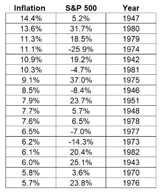
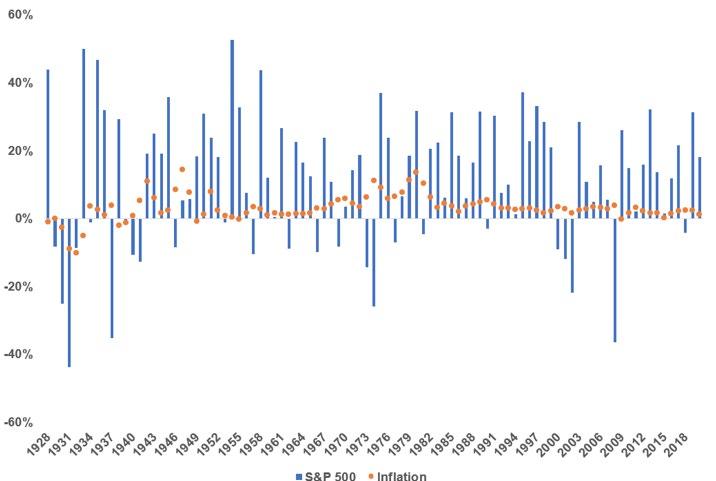 Figure 1: Stock Market vs. Inflation 1928 – 2020
Figure 2: Highest Annual Inflation Recordings
Figure 1: Stock Market vs. Inflation 1928 – 2020
Figure 2: Highest Annual Inflation Recordings
103
Source: Seeking Alpha
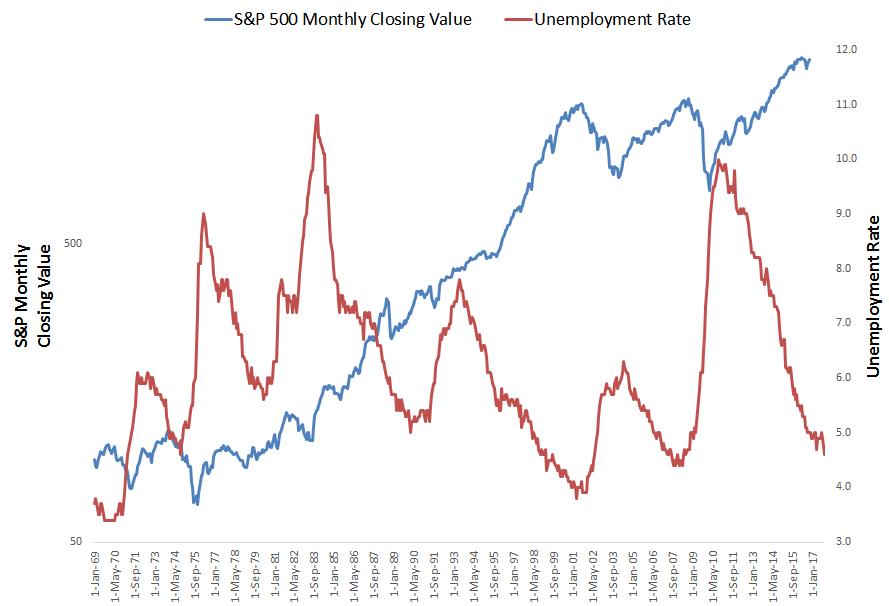
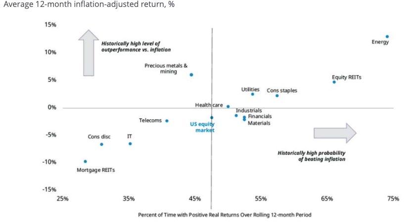 Figure 3: US Equity Sector Performance in High (+3% on Average) and Rising Inflation Environments, 1973-2022
Source: Hartford Funds
Figure 4: Unemployment Rate vs. S&P 500 Close
Figure 3: US Equity Sector Performance in High (+3% on Average) and Rising Inflation Environments, 1973-2022
Source: Hartford Funds
Figure 4: Unemployment Rate vs. S&P 500 Close
104
3. Literature Review
Inflation is a crucial factor that an alter stock market return, and numerous studies have attempted to explore the relationship between the two. The seminal study by Ammer (1994) examines the impact of inflation on stock returns, finding that higher inflation rates are associated with lower stock returns. This relationship is explained by inflation risk, which causes uncertainty among investors and leads them to demand higher returns to compensate for the additional risk.
Building upon Ammer's work, Alagidede and Panagiotidis (2010) investigate whether common stocks prove to be safe hedges against high levels of inflation. The authors find that the relationship between inflation and stock returns varies across countries and time periods, but there is some evidence to suggest that the stock market has patial hedging ability against inflation. However, this relationship is not significant in all cases, indicating that other factors may also play a role. Similarly, Li, Narayan, and Zheng (2010) analyze the how the stock market and inflation interact
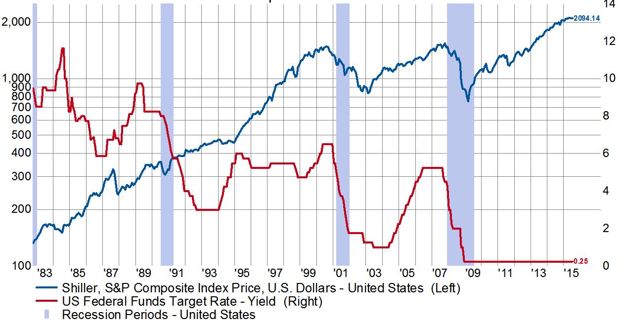 Figure 5: S&P 500 vs Federal Funds Rate
Source: Seeking Alpha
Figure 5: S&P 500 vs Federal Funds Rate
Source: Seeking Alpha
105
in the United Kingdom. The found a significant, negative relationship between inflation and stock market earnings. The authors suggest that this relationship may be due to the fact that inflation reduces the real value of future cash flows, making stocks less attractive to investors.
Oprea (2014) examines the Fisher Effect, which hypothesizes a positive effect of inflaiton on the stock market, and investigates its relevance for the Romanian stock market. The author finds that there is evidence of the Fisher Effect in the Romanian market, indicating that inflation expectations can affect stock prices. Bordo, Dueker, and Wheelock (2009) take a different approach by examining the relationship between monetary policy, inflation, and stock market conditions. Using a hybrid latent-variable VAR model, the authors find that monetary policy shocks have a significant impact on both inflation and stock market conditions. However, the relationship between inflation and stock returns is complex and depends on various factors such as the state of the economy and the monetary policy regime. The impact of inflation on stock prices has also been investigated in emerging markets, such as Pakistan and Brazil. Qamri, Haq, and Akram (2019) examine the effect of inflation on stock prices in Pakistan and find that inflation has a negative impact on stock prices. Similarly, Pimentel and Choudhry (2014) investigate the impact of high inflation and interest rates on stock returns in Brazil, finding that high inflation rates have a negative effect on stock returns.
Finally, Cohn and Lessard (1981) examine the impact of inflation on stock prices across several countries, finding a negative relationship between the two. Similarly, Boyd (1980) analyzes the effect of inflation on stock market returns, finding that the relationship between inflation and stock returns is negative, but the magnitude of the effect varies depending on the level of inflation. The literature provides ample evidence of a negative relationship between inflation and stock returns. Higher inflation rates are associated with greater inflation risk, which leads to uncertainty among investors and results in lower stock returns. While some studies suggest that stocks may provide a partial hedge against inflation, the relationship is not significant in all cases. Other factors such as monetary policy, inflation expectations, and the state of the economy may also play a role. These findings have important implications for investors and policymakers, who must carefully consider the impact of inflation on the stock market when making investment decisions and formulating monetary policy.
106
4.0 Data & Empirical Methodology
4.1 Data
The data that is used in this study comes from two main sources, Federal Reserve Economics Data (FRED) and Bloomberg. The dataset is a collective of monthly, time series data spanning from January 2012 to December 2022. The data consists of reports based in the Uninted States, with the S&P 500 as the main focus of the study. Table 1 represents the summary statistics of the varibales used in this study.
4.2 Empirical Model
My model is most similar in structure to that of study we followed the model from Ghulam Qamri et al. (2015) below:
With S representing Stock Price as the dependent variable, the model regresses inflation rate against stock price as the sole independent variable. The model that I used in this study was more complex than the one used by Qamri et al. (2015). My model is as follows:
�������������������� = ����0 + ����1 ���������������� + ����2
+ ����3 ���������������� + ����
STCK is the monthly cumulative stock market return of the S&P 500 index. I decided to use the S&P 500 as it gives a summarized insight into the entire stock market throughout the United
Count Mean Standard Deviation Minimum Maximum STCK 131 129.88 93.247 0.640 342.193 CPI 131 2.56 1.009 1.517 6.617 1 Year Expected Inflation 131 1.66 0.472 -0.219 2.824 Fed Funds Rate 131 0.73 0.91 0.05 4.10
Table 1: Summary Statistics
��������
������������������������������������
= ����0 + ����1
���������������� + ��������
��������������������−1
107
States. INF represents the consumer price index (CPI) measurements according to the U.S. Bureau of Labor Statistics. The CPI is one of the most common inflation measurements used by economists throughout empirical studies. Part of this study hypothesizes that expected inflation may have a more significant impact on stock market fluctuations compared to CPI measurements. Due to the stock markets resilience throughout economic turmoil, I theorized that the stock market may adjust and hedge losses due to inflation expectations. EINF represents 1 –year expected inflation from the Federal Reserve Economic Database (FRED). Finally, the model in this study include FIR as the federal interest rate for the period. Although our model is a more robust version of the one used by Qamri et al. (2015), the method that is used to regress the data resembles that of the empirical study done by Ammer (1994).
Ammer (1994) uses a vector autoregression to analyze his data. Due to our time-series data, and the way that past datapoints have a direct effect on future projections, a vecto autoregressive (VAR) model is neccesary. VAR models require a lag – length selection which is decided based on standardized tests and criteria. There are two criteria commonly refferenced when considering lag length of a model. The Akaike Information Criterion (AIC) and the Hannan Quinn (HQ) Criterion are the most common and in this model we tested our lag length refferring to them. Figure 6 represents the lag order selection criteria that was used in determing the lag length for this regression. In conjunction with a paper by Bekaert et al. (2009) the authors use six lag lengths. Figure 6 shows the recommendations of the AIC and HQ criterion, which ranges from two to seven lag periods. I decided to choose six lag periods for my model in conjunction with that of Bekaert et al. (2009). Figure 7 represents the Residual Serial Correlation LM Test that was carried out on the model ensuring that no serial correlation was present at the selected lag period.
108
Figure 6: VAR Lag Order Selection Criteria
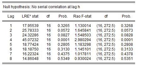
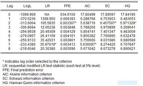
109
Figure 7: VAR Residual Serial Correlation LM Test
5.0 Empirical Results
The empirical results from the VAR on the dataset is presented in Table 2. The regression found a negative relationship between 1 year expected inflation and S&P 500 returns at three lag periods. The P-Value of the 1 year expected infaltion coefficient indicates a significance at the 5% significance level. The regression also found a negative relaitonship between the federal funds rate and S&P 500 returns at one lag period at the 10% significance level. The R-squared measurements for our variables are relatively high indicating accurate results within the regression analysis. Due to the nature of our time series dataset, it was necessary to run a Granger Causality test which is represented in Table 3. The Granger Causality test provided conflicting results from the regression for our model, indicating the CPI variable as the most causal in the model. The P-value from the causality test indicates that the CPI is significant at a 1% significance level.
Coefficient Std. Error t - statistic p - Value S&P 500 Growth (t-1) 0.751027 0.105607 7.11152 0.00001 *** 1 Year Expected (t-3) -53.69392 20.41562 -2.630041 0.0089 ** Federal Funds Rate (t-1) -19.83367 10.3551 -1.915353 0.0489 * S&P 500 Growth CPI 1 Year Expected Inflation Federal Funds Rate R-squared 0.98759 0.992 0.581888 0.986477 Adjusted Rsquared 0.98463 0.99022 0.482535 0.98326 110
Table 2: Vector Autoregression Results
Table 3: Granger Causality Test
5.0 Conclusion
In conclusion, stock market return is effected by all three of the independent variables that were tested in this model. In line with our hypothesis and the results found in the study by Li, Narayan, and Zheng (2010), this study finds that expected inflation and CPI inflation measurements have a significant negative impact on S&P 500 returns. The addition of the federal funds rate in to the model was beneficial as it was significant. According to the regression, an increase in the federal funds rate would lead to a decrease in stock market return. Increasing the federal funds rate is a common monetary policy decision made to slow down inflation, constriciting the economy. This was evident in the U.S. economy over the past two years, which was the inspiration for this paper. As the economy experienced high levels of inflation due to the pandemic and supply-chain issues, the Federal Reserve made the tough decision to increase interest rates. These increases have slowed the economy drastically and has led many to believe that the economy is currently in recession. Increased inflation and inflation expectations have a negative effect on stock market returns and the combination of increased interest rates could multipy the damge to investments, according to our study. This is a risk that investors and policy makers will monitor, factoring in many other factors such as unemployment and political instability.
Dependent Variable: Stock Market Return Excluded df P-value CPI 6 0.0097 1-Year Expected Inflation 6 0.8893 Federal Funds Rate 6 0.4682 All 18 0.0407
111
Works Cited
Alagidede, P. & Panagiotidis, T. (2010) Can Common Stocks Provide A Hedge Against Inflation? Journal of Risk Finance, 11(1), pp. 44-57.
Ammer, J. (1994) Inflation, inflation risk, and stock returns. Journal of Finance, 49(1), pp. 43-62.
Bordo, M. D., Dueker, M. J., & Wheelock, D. C. (2009) Inflation, monetary policy and stock market conditions: quantitative evidence from a hybrid latent-variable VAR. Journal of Business & Economic Statistics, 27(2), pp. 161-175.
Cohn, R. A. & Lessard, D. R. (1981) The Effect of Inflation on Stock Prices: International Evidence. Financial Analysts Journal, 37(1), pp. 41-46.
Li, L., Narayan, P. K. & Zheng, X. (2010) An analysis of inflation and stock returns for the UK. Applied Financial Economics, 20(8), pp. 609-618.
Muhammad Qamri, G., Abrar Ul Haq, M., & Akram, F. (2018) The Impact of Inflation on Stock Prices: Evidence from Pakistan. Pakistan Journal of Social Sciences (PJSS), 38(1), pp. 116.
Oprea, D. S. (2014) The Fisher effect: Evidence from the Romanian Stock Market. Romanian Economic Journal, 17(52), pp. 99-118.
Pimentel, R. C. & Choudhry, T. (2014) Stock Returns Under High Inflation and Interest Rates: Evidence from the Brazilian Market. International Review of Financial Analysis, 33, pp. 23-32.
Sathyanarayana, S. (2013) An Analytical Study of the Effect of Inflation on Stock Market Returns. International Journal of Marketing, Financial Services & Management Research, 2(4), pp. 90-104.
112
Carlson, B. (2021). Inflation vs. Stock Market Returns. A Wealth of Common Sense. Retrieved from https://awealthofcommonsense.com/2021/10/inflation-vs-stock-market-returns/
113
An Empirical Analysis of Foreign Trade and Institutional Quality on Economic Growth in Asian Countries
Ruixi Huanga
Abstract:
This investigation explores the connections between foreign commerce, institutional quality, and economic growth in 11 Asian nations, utilizing panel data spanning 2000 to 2021. The countries are classified into Central Asia and Southeast Asia groups. Economic growth serves as the dependent variable, while trade openness, FDI, institutional quality, human capital, and terms of trade act as independent variables. The outcomes reveal that only total life expectancy at birth significantly influences Central Asian countries' economic growth. Furthermore, trade openness, FDI net inflows, and governance indicators considerably affect Southeast Asian nations. The results also indicate that institutional quality's impact on economic growth is more pronounced in Southeast Asia.
JEL Classification: F43, O11,O53
Keywords: Economic Growth, Foreign Trade, Institutional Quality, Human Capital, Terms of Trade, Panel Data Analysis
a Bryant University, 1150 Douglas Pike, Smithfield, RI02917. Phone: +1(401) 757-9553.
Email:rhuang1@bryant.edu
114
I. Introduction
In recent decades, economic growth in the Asian region has been remarkable and has caught the attention of policymakers and scholars alike. Foreign trade and institutional quality are important indicators of a country's overall economic development. These indicators can capture diverse attributes of a country, including its degree of economic openness, competitiveness, stability, and overall governance quality (De Groot et al., 2004). Foreign trade represents a nation's economic policy, development stage, and natural resource availability, while institutional quality signifies the robustness and efficacy of its political and economic institutions (Carlsson & Stankiewicz, 1991). The Asian region has experienced remarkable economic growth in recent decades. This growth has been driven by a combination of factors, including trade liberalization, increased foreign investment, and improvements in the quality of institutions (Ocampo & Taylor, 1998). Therefore, this study is crucial for government to design effective policies to promote economic development in the Asian region.
Moving forward, The paper is structured as follows: Section II reviews relevant literature. Section III analyzes the economic trends in Southeast Asian and Central Asian countries. Section IV provides details on the data collection and methodology employed in this research. Section V presents the empirical results of the study. Finally, Section VI concludes the paper.
II. Literature Review
International trade fosters economic welfare by encouraging specialization and enabling countries to capitalize on their comparative advantage (Ruffin, 2002). Research has shown that open trade policies are linked to higher economic growth rates. Frankel and Romer (1999) found
115
that countries with open trade policies tend to experience greater economic growth. Moreover, Sun and Heshmati (2010) found that open trade policies were associated with economic expansion. Regarding institutional quality, Ahmed et al. (2022) identified its role in promoting economic growth in South Asian countries.
Increased trade openness can lead to gains in economic welfare by promoting specialization and allowing countries to benefit from their comparative advantage (Neary, 2007). Trade openness can also enhance productivity by facilitating the transfer of technology, knowledge, and capital across countries (Javorcik, 2004). In addition, FDI is an important source of capital for developing countries. FDI can have positive spillover effects on domestic firms, such as increased access to technology and knowledge, improved management practices, and higher productivity (Blomstrom and Kokko, 1998).
Additionally, strong institutional quality can foster economic growth by decreasing transaction costs, enhancing contract enforcement, and stimulating investment (Acemoglu et al., 2001). Supporting this notion, Knack and Keefer (1995) discovered that nations with superior institutional quality witnessed higher economic growth rates after analyzing data from 60 developing countries. In a parallel vein, Mauro's (2002) research on corruption and economic growth, which examined data from 41 developing nations, unveiled that corruption negatively affects economic growth, with countries exhibiting lower levels of corruption typically experiencing higher growth rates.
Moreover, a well-educated and proficient workforce can bolster economic growth by enhancing productivity and facilitating the adoption of innovative technologies (Lucas, 1988). Numerous empirical investigations have established that human capital can stimulate economic
116
growth in developing nations, including those in Asia (Mankiw et al., 1992; Barro, 1997; Benhabib and Spiegel, 2005). Additionally, alterations terms of trade can impact economic growth by affecting the external balance and capacity to import essential capital goods and advanced technology (Sachs and Warner, 1995). Correspondingly, various studies have identified a correlation between advancements in terms of trade and economic growth within Asian countries (Sachs and Warner, 1995; Cashin et al., 2004).
III. Trend
Figures 1 and 2 display the annual GDP per capita growth rate of South East Asian and Central Asian countries from 2000 to 2021. Both regions experienced mostly positive growth rates throughout this period, with some year-to-year fluctuations. Notably, Central Asian countries generally had higher GDP per capita growth rates. In 2020, both regions suffered a decline due to the COVID-19. The global financial crisis in 2009 also caused a downturn for South East Asian countries. The highest GDP per capita growth rate for South East Asian countries occurred in 2010 (6.41%), while for Central Asian countries, it was in 2004 (7.25%).
Figure 1: GDP per capita growth rate in Southeast and Central Asian Countries
-10 -5 0 5 10 2000 2001 2002 2003 2004 2005 2006 2007 2008 2009 2010 2011 2012 2013 2014 2015 2016 2017 2018 2019 2020 2021 GDP per capita growth rate(%) in Southeast and
South East Asian countries Central Asian countries 117
Source: Author’s calculation by World Bank database
Central Asian Countries
Figure 2
GDP per capita growth rate (%) in Southeast and Central Asian Countries
Author’s calculation by World Bank database Figure 3 and Figure 4 show the gross fixed capital formation for Central and Southeast Asian countries between 2000 and 2021. From the graph, both regions experienced fluctuations in gross fixed capital formation between 2000 and 2021. Central Asian countries experienced a sharp increase in gross fixed capital formation from 2000 to 2009, while Southeast Asian countries experienced insignificant growth. Between 2002 and 2009, the gross fixed capital formation in Southeast Asian countries exceeded that of Central Asian countries. However, from 2014 to 2021, the opposite trend was observed, with Central Asian countries experiencing higher gross fixed capital formation than their Southeast Asian counterparts. This indicates a significant shift in investment trends and priorities between the two regions over time. During the earlier period, Southeast Asian countries may have prioritized infrastructure development and investment, resulting in higher gross fixed capital formation. In contrast, Central Asian countries may have been focused on other economic sectors during that time. In the more recent period, Central Asian countries have increased their investment in fixed capital, indicating a renewed
-10 0 10 2000 2001 2002 2003 2004 2005 2006 2007 2008 2009 2010 2011 2012 2013 2014 2015 2016 2017 2018 2019 2020 2021
Source:
118
South East Asian countries Central Asian countries
focus on infrastructure and economic development. This may be due to factors such as increased government spending, favorable investment climate, or improved economic policies. In 2020, both regions experience a decline as a result of COVID-19. In 2021, Southeast Asian countries experienced a slight increase in gross fixed capital formation while Central Asian countries experienced a slight decrease.
Overall, it is suggested that Central Asian countries have been increasing their investment in fixed capital over the past decade, while Southeast Asian countries have seen a decline in their investment in fixed capital during the same period. However, both regions have been affected by COVID-19, with a slight recovery seen in 2021.
Figure 3: Gross fixed capital formation in Southeast and Central Asian Countries
0 10 20 30 40 2000 2001 2002 2003 2004 2005 2006 2007 2008 2009 2010 2011 2012 2013 2014 2015 2016 2017 2018 2019 2020 2021 Gross fixed capital formation (% of GDP) South East Asian countries Central Asian countries 119
Source: Author’s calculation by World Bank database
Gross Fixed Capital Formation(% of GDP)
Figure 5 presents the governance indicators for Central Asia and Southeast Asia from 2000 to 2021. The overall governance metric employed here is derived from the average of six integral components. From 2005 to 2008, the governance indicator for both regions remained relatively stable, with Southeast Asian countries maintaining a higher indicator than Central Asian countries. However, there was a significant increase in the governance indicator for Central Asian countries in 2009, while that of Southeast Asian countries remained relatively the same. From 2010 to 2014, the governance indicators for both regions continued to increase, with South East Asian countries maintaining a higher indicator than Central Asian countries. In 2014, both regions recorded significant increases in their governance indicators, with Central Asian countries having a higher indicator than South East Asian countries. In 2021, there was a significant increase in the governance indicator for Central Asian countries, while that of Southeast Asian countries remained relatively stable.
Figure 4:
Source: Author’s calculation by World Bank database
0 10 20 30 40 2000 2001 2002 2003 2004 2005 2006 2007 2008 2009 2010 2011 2012 2013 2014 2015 2016 2017 2018 2019 2020 2021
120
South East Asian countries Central Asian countries
Looking at the individual indicators, the Central Asian Countries have consistently scored lower than the Southeast Asian Countries across all indicators. The Southeast Asian Countries scored higher in these indicators, as well as in the Government Effectiveness indicator. Overall, the graph shows that the governance indicators for both regions have fluctuated over time, with Southeast Asian countries generally having higher indicators than Central Asian countries. Also, both regions have made progress in their governance indicators over time, although there is still room for improvement.
Source: Author’s calculation by World Bank database
Data and Empirical Methodology
1. Data
The study utilizes panel data, which means that data is collected over time from multiple observations (in this case, 11 Asian countries) to examine trends and patterns in the data. The data is divided into two groups, Central Asia and Southeast Asia. The data utilized in the study is
Figure 5
0 20 40 60 80 100 2000 2001 2002 2003 2004 2005 2006 2007 2008 2009 2010 2011 2012 2013 2014 2015 2016 2017 2018 2019 2020 2021 Goverance indicators(Region Average) Central Asian Countries South East Asian Countries 121
sourced from the World Bank Database, which is a widely used and reliable source of data for economic research. Tables 1 and 2 likely present the variables used in the study, as well as summary statistics for these variables.
Source: Author’s calculation using STATA output
In summary, the data presented in Table 1 indicates that Central Asia has a somewhat open economy, with notable disparities in GDP per capita and foreign direct investment. Life expectancy is relatively low, and there is room for enhancement in governance scores. However, the net barter terms of trade suggest that the region has a positive trade balance.
Variables Obs Mean Std. dev. Min Max GDP per capita growth rate 88 4.297436 3.407952 -10.12045 13.69319 Trade openness 88 0.854061 0.3184702 0.291923 1.753512 FDI, net inflows 88 2.21E+09 3.99E+094.02E+08 1.72E+10 Life expectancy at birth 88 68.68366 2.172458 63.26 73.18 Net barter terms of trade index 88 131.0819 39.261 82.69491 223.506 Governance indicator 88 20.43568 9.514773 5.921952 42.2679
Table 1 (Central Asian) Summary Statistics
122
Table 2 (South East Asian) Summary Statistics
The data presented in Table 1 offers an insight into the economic and social landscape of Central Asia, revealing a region that possesses a moderately open economy. However, there is a marked variation in GDP per capita and foreign direct investment, indicating that the economic situation differs widely between the countries in the region. Additionally, the average life expectancy is relatively low, which is an area of concern that requires attention. Governance scores also suggest that there is ample room for improvement, indicating a need for more effective policies and institutions to foster growth and stability. On a positive note, the net barter terms of trade indicate that Central Asia has a favorable trade balance, which is a promising development for
Variables Obs Mean Std. dev. Min Max GDP per capita growth rate 154 3.694436 3.17404210.97819 12.50852 Trade openness 154 1.480909 0.9771644 0.329756 4.373267 FDI, net inflows 154 1.32E+10 2.03E+104.95E+09 1.11E+11 Life expectancy at birth 154 73.05471 4.851978 58.625 83.7439 Net barter terms of trade index 154 98.89924 17.197 66.59283 138.0932 Governance indicator 154 47.20632 20.12576 19.63838 89.89646
Source: Author’s calculation using STATA output
123
the region. This suggests that the region is able to generate revenue from its exports and is not overly reliant on imports.
2. Correlation Analysis
Table 3 displays the Pearson correlation coefficient for each variable in Central Asian countries.
A positive correlation coefficient for Trade Openness suggests a positive association with GDP per capita in these nations. Conversely, the negative correlation coefficients for Foreign Direct Investment, Net Barter Terms of Trade Index, and Governance Score imply a weak negative relationship with GDP per capita.
* p<0.05 ** p<0.01
Source: Author’s calculation using STATA output
Table 4 displays the correlation between GDP per capita and the variables in South East Asian Countries, along with the corresponding Pearson correlation coefficient for each variable. In addition, life expectancy was negatively correlated with GDP per capita with a correlation coefficient of -0.2412. This may be due to factors such as environmental pollution or lifestyle
Table 3: Central Asian correlation
Pearson GDP per capita growth Trade Openness 0.174 FDI, net inflows -0.1 Net barter terms of trade index -0.536 Life expectancy at birth -0.117 Governance indicator -0.273
Table 3: Central Asian Correlation
124
changes. Besides, there is a positive correlation between the net barter condition and the economic development of the region with a correlation coefficient of 0.0416. Furthermore, the quality of governance is negatively correlated with GDP per capita with a correlation coefficient of -0.1712. This may be due to factors such as corruption or concentration of power in the hands of a few individuals.
* p<0.05 ** p<0.01
Source: Author’s calculation using STATA output
3. Empirical Model
The subsequent model incorporates all explanatory variables and governance indicators for estimation:
Dependent Variable: GDP per capita growth rate, serving as a proxy for economic growth rate.
Independent Variables: TOit – Trade Openness, measured by the ratio of the sum of imports and exports to the country's GDP in the corresponding period. FDIit- foreign direct investment (net
Pearson GDP per capita growth(annual %) Trade Openness 0.0054 FDI, net inflows 0.0099 Net barter terms of trade index 0.0416 Life expectancy at birth -0.2412 Governance indicator -0.1712
Table 4: South East Asian correlation
Table
4: South East Asian Correlation
Economic growth= ����0 + ����1TOit + ����2FDIit + ����3IQit + ����4HCit+ ����5TTRADEit + Ꜫ (1)
125
flows), representing the net inflow of investment to obtain a lasting management interest in an enterprise that operates in an economy different from that of the investor. IQit- Institutional Quality, comprising six governance indicators: Control of Corruption, Government Effectiveness, Political Stability and Absence of Violence, Regulatory Quality, Rule of Law, and Voice and Accountability. Overall governance, the average of these six indicators, is used to represent institutional quality in this paper. HCit- Human Capital, with Life Expectancy serving as a proxy. TTRADEit- Terms of Trade, using Net barter trade as a proxy.
IV. Empirical Results
Table 5 presents the empirical findings of a linear regression model with five independent variables. The dataset used for the regression analysis consists of 88 observations for Central Asian countries and 154 observations for Southeast Asian countries.
Variables Central Asian Southeast Asian Intercept 65.6543 (5.1976) 22.3903*** (3.9270) Trade Openness -0.1915 (-0.1662) 1.6649*** (3.7926) FDI, net inflows -7.9731 (-0.6773) 4.0969* (2.4942) Life expectancy at birth -0.9106* (-4.8377) -0.2860** (-3.3112) Net barter terms of trade index 0.01487 (1.3740) 0.0221 (1.5497) 126
Table 5: Regression results for Central Asian and Southeast Asian
The values in parentheses are T values * P< 0.05 **P< 0.01 ***P< 0.001
Source: Author’s Calculations using STATA output
For Central Asian Countries, the overall regression model is statistically significant as the probability value is 0.0000 This demonstrate that the independent variables significantly impact economic growth. The Trade Openness coefficient is negative (-0.1915) but not statistically significant (p-value = 0.868). Similarly, the Foreign Direct Investment Net Inflows coefficient is negative (-7.97e-11) and not statistically significant (p-value = 0.500), implying no significant relationship with economic growth. The Net Barter Terms of Trade coefficient is positive (0.0149) but not statistically significant (p-value = 0.173). The Governance Indicators coefficient is negative (-0.0208) but not statistically significant (p-value = 0.656). Furthermore, the coefficient for Life Expectancy at Birth Total in the regression analysis is negative, indicating a downward trend (-0.9106).
This finding may indicate that factors such as inadequate health care, limited access to education, and poverty can limit economic development. Nations with higher life expectancies might have a larger aging population, which could diminish the labor force and productivity. Furthermore, healthcare costs may rise with an aging population, potentially straining government budgets and reducing funds for other areas that could foster economic growth.
Governance indicator -0.0207 (-0.4464) -0.0636* (-2.4418) R2 0.3103 0.1848 Adjusted R2 0.2682 0.1573 F-statistics F(5,82)= 7.3784, p=0.0000 F(5,148)= 6.7107, p=0.0000 Number of obs. 88 154
127
Ultimately, only life expectancy at birth total emerged as a statistically significant predictor of GDP per capita growth in these countries. Other factors, such as trade openness, foreign direct investment net inflows, net barter terms of trade index, and governance indicators, do not seem to significantly influence economic growth. In Central Asian countries, inadequate infrastructure, political instability and a shortage of skilled labor limit trade economic growth. As a result, these variables may not have a statistically significant influence on the region's economic growth, despite their recognized importance in economic theory.
Inadequate infrastructure in Central Asia can limit the ability of foreign investors to gain a foothold in the region. Additionally, political instability and regional conflicts can dissuade foreign investors and limit trade opportunities, ultimately dampening the potential economic benefits. Furthermore, the shortage of skilled labor in Central Asia may limit the ability of the region to maximize the benefits of foreign direct investment and trade openness. Without an adequate workforce, the potential benefits of these variables may not translate into sustainable economic growth.
For Southeast Asian countries, The model had an F-value of 6.71 and a P-value of 0.0000, indicating that the entire model was statistically significant. the R-squared was 0.1848.
Regression analysis shows that trade openness and FDI have a significant impact on economic growth in Southeast Asia. The analysis suggests a significant correlation between trade openness, net inflows of FDI, and economic growth. However, the results also show a negative and statistically significant coefficient (with a p-value of 0.016) between Governance Indicators and GDP per capita growth in Southeast Asian countries. This indicates that better governance may be a crucial factor for promoting economic growth in Southeast Asia. However, the coefficients
128
for
Life Expectancy at Birth Total and Net Barter Terms of Trade Index are negative but not statistically significant (p-value > 0.05), indicating that these variables do not substantially impact economic growth in this region.
The regression results for Southeast Asian countries suggest that trade openness, foreign direct investment and governance indicators play an important role in driving economic growth in Southeast Asia. Governments in this region can implement measures to boost trade openness, attract more FDI inflows, and enhance governance quality to promote economic growth.
Furthermore, the study reveals that life expectancy at birth and net barter terms of trade index do not significantly impact economic growth in these countries. This finding suggests that governments should prioritize improving factors such as trade openness, FDI inflows, and governance quality, rather than solely focusing on enhancing life expectancy or terms of trade, to foster economic growth.
Thus, for the Central Asian countries, only total life expectancy at birth has a significant negative correlation with economic growth. The findings suggest that factors such as inadequate healthcare, limited access to education, and poverty may be contributing to slower economic growth in the region. To address these challenges, governments in Central Asia should focus on improving healthcare, education, and poverty alleviation measures. On the other hand, for Southeast Asia, the regression results emphasize the impact of trade openness, FDI and governance indicators on economic growth. Life expectancy and net barter terms of trade index do not appear to be significant determinants of economic growth in Southeast Asia. As a result, Southeast Asian governments should prioritize enhancing trade openness, attracting more FDI inflows, and improving governance quality to stimulate economic growth, rather than solely concentrating on life expectancy or terms of trade.
129
V. Conclusion
In conclusion, this study highlights the important factors that influence economic growth in Central and Southeast Asia. While life expectancy is the only significant predictor in Central Asian countries, trade openness and FDI inflows are crucial factors for stimulating economic growth in Southeast Asian countries. The study emphasizes the importance of improving healthcare, education, and poverty alleviation measures in Central Asia to overcome the challenges that limit economic growth. In Southeast Asia, the focus should be on enhancing trade openness, attracting more FDI inflows, and improving governance quality.
The regression analyses demonstrate that foreign trade and institutional quality are crucial determinants of economic growth in both Central and Southeast Asian countries. Specifically, in Central Asian countries, the results suggest that only life expectancy at birth significantly affects GDP per capita growth, exhibiting a negative relationship. This implies that efforts to enhance healthcare and reduce mortality rates could contribute to the region's economic growth. In Southeast Asian countries, trade openness, FDI, life expectancy at birth, and governance indicators have significant impact on economic growth. These findings indicate that Southeast Asian countries could foster their economic growth by focusing on improving foreign trade and investment, healthcare, and institutional quality.
Based on these insights, it is recommended that governments in both Central and Southeast Asian countries focus on policy measures that encourage trade openness, attract foreign direct investment, enhance healthcare, and bolster institutional quality. This could encompass initiatives such as investing in healthcare infrastructure and education, minimizing trade barriers, refining regulatory frameworks, and boosting transparency and accountability in governance (Swinburn et al., 2015).
130
Acemoglu, D., Johnson, S., & Robinson, J. A. (2001). The colonial origins of comparative development: An empirical investigation. American economic review, 91(5), 13691401.
Ahmed, F., Kousar, S., Pervaiz, A., & Shabbir, A. (2022). Do institutional quality and financial development affect sustainable economic growth? Evidence from South Asian countries. Borsa Istanbul Review, 22(1), 189-196.
Barro, R. J. (1997). Determinants of economic growth.
Benhabib, J., & Spiegel, M. M. (2005). Human capital and technology diffusion. Handbook of economic growth, 1, 935-966.
Blomström, M., & Kokko, A. (1998). Multinational corporations and spillovers. Journal of Economic surveys, 12(3), 247-277.
Carlsson, B., & Stankiewicz, R. (1991). On the nature, function and composition of technological systems. Journal of evolutionary economics, 1, 93-118.
Cashin, P., Liang, H., & McDermott, C. J. (2000). How persistent are shocks to world commodity prices?. IMF Staff Papers, 47(2), 177-217.
De Groot, H. L., Linders, G. J., Rietveld, P., & Subramanian, U. (2004). The institutional determinants of bilateral trade patterns. Kyklos, 57(1), 103-123.
Frankel, J. A., & Romer, D. (1999). Does trade cause growth?. American economic review, 89(3), 379-399.
BIBLIOGRAPHY
131
Javorcik, B. S. (2004). The composition of foreign direct investment and protection of intellectual property rights: Evidence from transition economies. European economic review, 48(1), 39-62.
Knack, S., & Keefer, P. (1995). Institutions and economic performance: cross‐country tests using alternative institutional measures. Economics & politics, 7(3), 207-227.
Lucas Jr, R. E. (1988). On the mechanics of economic development. Journal of monetary economics, 22(1), 3-42.
Mankiw, N. G., Romer, D., & Weil, D. N. (1992). A contribution to the empirics of economic growth. The quarterly journal of economics, 107(2), 407-437.
Mauro, P. (2004). The persistence of corruption and slow economic growth. IMF staff papers, 51(1), 1-18.
Neary, J. P. (2007). Cross-border mergers as instruments of comparative advantage. The Review of Economic Studies, 74(4), 1229-1257.
Ocampo, J. A., & Taylor, L. (1998). Trade liberalisation in developing economies: modest benefits but problems with productivity growth, macro prices, and income distribution. The Economic Journal, 108(450), 1523-1546.
Romer, P. M. (1986). Increasing returns and long-run growth. Journal of political economy, 94(5), 1002-1037.
Romer, P. M. (1990). Endogenous technological change. Journal of political Economy, 98(5, Part 2), S71-S102.
Ruffin, R. (2002). David Ricardo's discovery of comparative advantage. History of political economy, 34(4), 727-748.
132
Sachs, J. D., Warner, A., Åslund, A., & Fischer, S. (1995). Economic reform and the process of global integration. Brookings papers on economic activity, 1995(1), 1-118.
Solow, R. M. (1956). A contribution to the theory of economic growth. The quarterly journal of economics, 70(1), 65-94.
Sun, P., & Heshmati, A. (2010). International trade and its effects on economic growth in China.
Swinburn, B., Kraak, V., Rutter, H., Vandevijvere, S., Lobstein, T., Sacks, G., ... & Magnusson, R. (2015). Strengthening of accountability systems to create healthy food environments and reduce global obesity. The Lancet, 385(9986), 2534-2545.
133
An Empirical Analysis of the Impact Specific Crimes Have on Property Values in Massachusetts
Jack Scott
Abstract:
This research paper examines the impact of specific crime types on property values in urban areas. Using a dataset of property sales and crime data from several cities in Massachusetts, a regression analysis is applied to estimate the effect of different crime types on property values. Our findings suggest that certain types of crime, such as violent crimes and drug-related offenses, have a significant negative impact on property values, while other types of crime, such as property crimes and white-collar crimes, have a relatively small effect on property values. We also find that the effect of crime on property values varies across different neighborhoods and is influenced by factors such as socioeconomic status of the neighborhood. These results have important implications for policymakers and urban planners seeking to improve public safety and promote economic development in urban areas.
JEL Classification(s): R30, R31, R51, R58, R11, R21
Keywords: Real Estate, Property Values, Crime
Department of Economics, Bryant University, 1150 Douglas Pike, Smithfield, RI 02917. Email: jscott11@bryant.edu
134
The real estate market is a critical component of the economic health and financial stability of any nation. Property values are influenced by a multitude of factors such as the health of the real estate market itself, a property’s location, the socioeconomic makeup of the surrounding area, interest rates, and the size and condition of the property. It is also well documented that crime has a significant impact on the value of real estate. The objective of this study is to enhance the understanding and to fill the gaps in previous literature of the impact specific crimes have on home values. Previous studies have shown that there is a significant correlation between the crime rate of an area and the property values in that specific area. The objective of this paper is to determine if specific crimes have a greater impact on property values than others.
From a policy perspective, this analysis is important for several reasons. Crime is a major concern for policy makers. Reducing crime is imperative for economic growth and stability. Understanding what crimes have the greatest impact on property values allows policymakers to formulate strategies to reduce specific crimes and promote community, economic, and social prosperity. As Massachusetts has been in a prolonged battle with opiate overdoses, this provides a unique opportunity to examine the impact that drug crimes have on residential property values. Furthermore, by understanding the impact specific crimes have on property values, local and federal resources can be allocated more efficiently to both combat crime and encourage economic development.
This paper was guided by several research objectives that are unique when compared to previous publications. Much of the literature on this topic is outdated. Local socioeconomic conditions evolve with time; therefore, literature on this subject becomes outdated and irrelevant quickly. Furthermore, as technology advances, so do criminals and the crimes they commit. There are many crimes that were not conceivable when previous literature on the subject was published. By using current cross section data published by the FBI, this study brings the most current and up to date data, solving the obsolescence of previous literature. There is a significant amount of literature published on one specific type of crime, for example sexually related crimes or drug related offenses, and their impact on property values. However, there is no current research that accounts for a variety of crimes. Finally, given the uncertainty facing the US real
1.0 Introduction
135
estate market caused by macroeconomic trends, this paper provides timely insight to a current event.
The rest of this paper is organized in the following order. The second section is a literature review of previously published and related research. Section three is a review of the empirical models and various regressions. In section four, the data used in these models as well as the methodology used are discussed. Section five discusses the results of the empirical models, which is followed by a conclusion in section six.
2.0 Literature Review & Industry Trends
Figure one (1) shows that the transaction costs of residential real estate in Massachusetts has seen steady increases since the financial crisis of 2008. Given the growth of home prices in Massachusetts, it is imperative to understand the past performance of residential real estate values before conducting analysis.
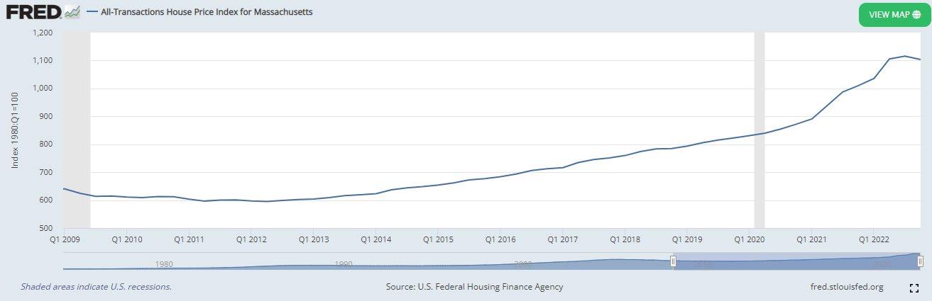
Source: FRED
According to the National Association of Realtors (NAR), the real estate industry in Massachusetts accounts for $105.8 billion or 16.6% of the state’s gross product in 2021. This is a significant portion of Massachusetts’ economy, and further supports the importance of researching the intricacies that affect real estate prices.
Figure 1: Home Price Index for Massachusetts (2009 – 2022)
136
There are also many macroeconomic factors that contribute to real estate prices. As shown in figure two (2), the Federal Reserve has raised the federal funds rate sharply after near zero levels since during the Covid-19 pandemic.
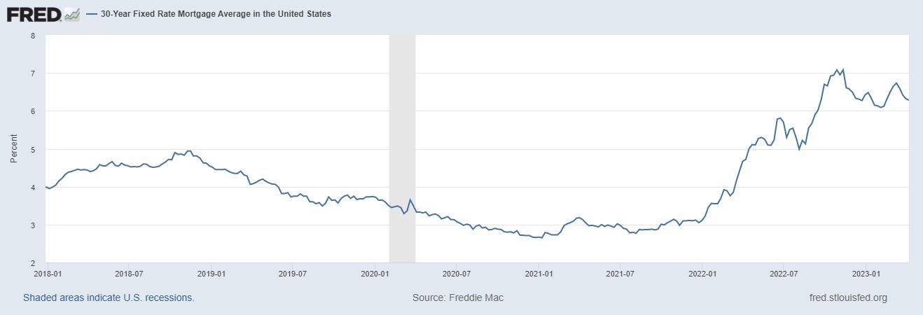
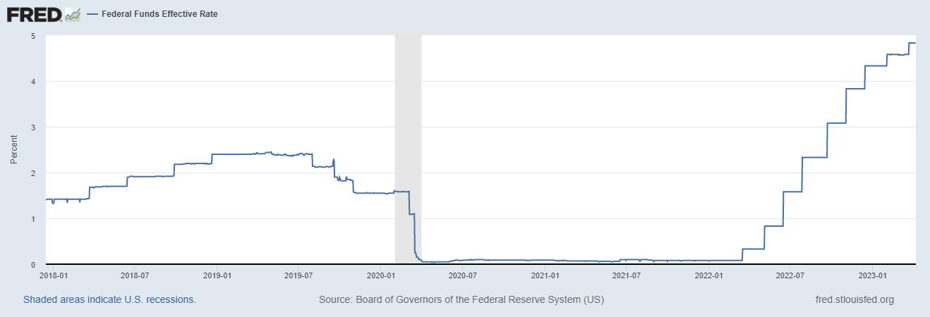
Source: FRED
The increased federal funds rate has led to increases in the price of debt. This is visualized in figure three (3), which shows the average 30-year fixed mortgage rate in the United States. Because it represents the cost of borrowing money, the 30-year fixed mortgage rate is seen as a useful indicator for the real estate industry. When mortgage rates are low, borrowing money to buy a home becomes cheaper, which can stimulate demand for real estate and increase home prices. When mortgage rates are high, it can make purchasing a property more expensive and reduce demand, resulting in lower home prices.
Source: FRED
Figure 2: The Federal Funds Rate (2018 – 2023)
Figure 3: 30 Year Fixed Mortgage Rates in the US (2018-2023)
137
The impact that crime has on real estate prices is well documented. However, cross sectional data that is current has not been applied to previous studies. Figure four (4) shows drug related arrest data. According to the FBI, a majority of drug related arrests in Massachusetts are related to opioids. Previous research shows that there is a correlation between increased opioid activity and a decrease in home values (Custodio et al., 2021).
There is also research that supports sexually related crimes have a statistically significant impact on real estate prices. Megan's Law is a federal statute in the United States that mandates states to set up a system for publicly disclosing information about registered sex offenders to safeguard communities and prevent sexual crimes. Megan Kanka, a seven-year-old girl who was abducted, raped, and killed by a known child molester who lived across the street from her family, inspired the law. Megan's Law requires convicted sex offenders to register with their local law enforcement authorities and allows the public to learn their identify, whereabouts, and criminal history. The law is intended to arm individuals with the information and resources they need to defend themselves and their families against sexual predators. The passing of this law was proven to have a significant impact on home values (Linden et al., 2007). It has been demonstrated that the values of homes within 0.1 miles of an offender see a 4% decrease in value. However, this effect dissipates rapidly with distance of homes from the offender as homes greater than 0.1 miles away see no negative impact (Tita et al., 2006; Buck et al., 1993).
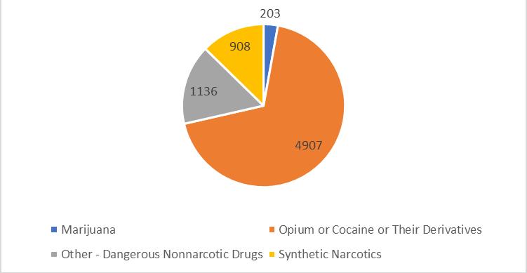 Figure 4: 2021 Drug arrests by category in Massachusets
Source: Federal Bureau of Investigation – Crime Data Explorer
Figure 4: 2021 Drug arrests by category in Massachusets
Source: Federal Bureau of Investigation – Crime Data Explorer
138
While the relationship between crime and real estate prices is well documented, many studies on the matter are antiquated and their data would not be applicable in the 21st century. However, the methodology applied by the authors to conduct their research is valuable. It is apparent that crime rates unanimously have a negative effect on the real estate industry. Additionally, there is strong evidence that crime of all types has a significant negative impact on market rent. The level of impact that violent crime has on housing prices is dependent on the socioeconomic makeup of the area (Rizzo, 1979; Naroff et al., 1980; Burnell, 1988).
4.0 Data and Empirical Methodology
4.1 Data
This study uses cross section data from 2022. All crime data was gathered from the Federal Bureau of Investigation (FBI)’s Crime Data Explorer. This data is updated annually and is publicly available to all. The dataset consists of 66 unique statistics for every city, town, and academic institution in Massachusetts. These statistics were then grouped to provide the most accurate and complete analysis. These groupings consist of assault offenses, loss of life (homicide, justifiable homicide, and manslaughter), sex crimes, burglary / breaking and entering, fraud, and weapons violations.
All home price data was collected from the NAR. Compiling monthly market reports for every town in Massachusetts for 2022, an average home price for each town was computed as well as the population for every town in Massachusetts. Given that there is a high likelihood that areas with greater populations will experience a larger amount of crime, the total amount of crimes committed was divided by the town’s population to compute each town’s crime rate. Additionally, median household income and per capita income were collected for each town using the most up to date census information for Massachusetts.
Finally, The FBI provided three additional groupings for crime data. These groups are: crimes against persons, crimes against property, and crimes against society. By utilizing both broad and specific groupings, the likelihood of accuracy is increased.
139
4.2 Empirical Model
Pulling inspiration from Ihlandfeldt and Mayock (2009), this model relied on a cross section of crime and housing data as well as controlling for population discrepancies.
Independent variables are directly from the FBI’s report or a computation from data sourced from the NAR and the census.
5.0 Empirical Results
The first regression results are below in table one (1). Given that socioeconomic conditions, populations, and property values are not uniform throughout each town in Massachusetts, towns were grouped by size. Table one consists of all cities and towns in Massachusetts. This was a preliminary regression that served as a proof of concept and to weigh the impact that income and population had on property values to ensure accurate information in future regressions.
���������������� �������������������� = ����0 + ����1 �������������������� ���������������� + ����2 ���������������������������� �������������������������������� + ����3 ���������������� �������� ���������������� + ����4 ������������ ������������������������ + ����5 �������������������������������� �������� �������������������������������� ������������ �������������������������������� + ����6 �������������������� + ����7 ���������������� �������������������������������� + ����8 ���������������������������� ���������������������������������������� + ����
Home Price = β0+ β1 Population+β2 Per Capita Income+ε SUMMARY OUTPUT Regression Statistics Multiple R 0.76391653 R Square 0.583568465 Adjusted R Square 0.580237013 Standard Error 260800. 1308 Obs ervations 253 ANOVA df SS MS F Significance F Regression 2 2.38289E+131.19144E+13175.16939032.77301E-48 Residual 2501.70042E+1368016708243 Total 2524.08331E+13 Coefficients Standard Error t Stat P-value Intercept -261718.19651264.32609-5.1052694146.54851E-07 Population 0.7827730890.3333541272.3481727810.019645646 Per capita Income 22.85017891.22201466718.69877632.10979E-49 140
Table 1: Preliminary Regression:
This model shows the impact that income and population have on home values in Massachusetts. An adjusted R2 of 0.58, given the simplicity of the model, paved the way for the final models used in this paper.
These findings lead to the conclusion that areas with higher population densities are prone to higher crime rates. For the model to be accurate, these findings must be accounted for. Table two (2) considers the population of cities and towns in Massachusetts. This model includes the 25 largest cities and towns in Massachusetts.
SUMMARY OUTPUT
Table 2: 25 Largest Cities in MA by population
Regression Statistics Multiple R 0.820648004 R Square 0.673463146 Adjusted R Square 0.469415843 Standard Error 460430.8339 Observations 25 ANOVA df SS MS F Significance F Regression 7 8.74461E+11 1.24923E+11 0.58927 0.749332274 Residual 2 4.23993E+11 2.11997E+11 Total 9 1.29845E+12 Coefficients Standard Error t Stat P-value Intercept 691301.9066 355980.4043 1.941966182 0.19164 Assault Offenses 174.300439 596.037501 0.292432001 0.7975 Loss Of Life69705.94984 71530.429950.974493651 0.43259 Sex Crimes 2414.699395 7522.848755 0.320982047 0.77866 Burglary / B&E3351.219757 2003.9975361.672267404 0.23644 Fraud Offenses 2243.61168 1549.787611 1.447689777 0.28467 Drug Offences1387.768818 2555.5741120.543036029 0.64153 141
It is well documented that crime has a negative impact on property values. The objective of this research was to prove a correlation between specific crimes and their impact on property values. This model shows that specific crimes have significantly more impact on property values in the densely populated areas of Massachusetts. Crimes that result in the loss of life such as murder or manslaughter, burglaries, and drug related offences are the largest contributors to crime’s negative impact on real estate values.
Moreover, this research also highlights the need for homeowners, real estate agents, and investors to consider crime rates when making decisions related to property purchases and sales.
It is essential to recognize that the value of a home is not only determined by its physical characteristics but also by its location and the safety of the surrounding area. As such, it may be wise for stakeholders to invest in preventative measures and community-building initiatives that aim to reduce crime rates in high-risk neighborhoods.
Finally, it is worth noting that this study focused specifically on densely populated areas in Massachusetts, and therefore, caution should be exercised when generalizing these results to other regions or different types of communities. Nonetheless, the findings of this research contribute to the growing body of literature on the economic impact of crime and provide important insights into the relationship between crime and property values in urban settings.
5.0 Conclusion
The above model has proven that crimes such as murder, burglary, and drug-related offenses significantly lower house prices. For legislators, law enforcement personnel, and community leaders who are concerned in improving public safety and establishing stable and flourishing communities, this study's findings have important implications. The findings of this study imply that lowering crime rates in these groups may lower housing costs.
This research also highlights the need for homeowners, real estate agents, and investors to consider crime rates when making decisions related to property purchases and sales. It is essential to recognize that the value of a home is not only determined by its physical
Weapon Law Violations 2382.638061 3284.860665 0.725339156 0.54363
142
characteristics but also by its location and the safety of the surrounding area. Therefore, it should be encouraged for those in the industry to invest in preventative measures and communitybuilding initiatives that would not only benefit themselves, but the community as a whole.
Finally, it is important to note that this study is specifically focused on areas in Massachusetts with the largest populations. Therefore, further research would be needed to be able to generalize these results to other communities, regions, and states.
Bibliography
Buck, Andrew J., and Simon Hakim. “Are Property Values Being Adversely Affected by Crime?” Journal of Property Valuation and Investment, vol. 9, no. 1, 1993, pp. 37–44., https://doi.org/10.1108/eum0000000003296.
Burnell, James D. “Crime and Racial Composition in Contiguous Communities as Negative Externalities: Prejudiced Household's Evaluation of Crime Rate and Segregation Nearby Reduces Housing Values and Tax Revenues.” American Journal of Economics and Sociology, vol. 47, no. 2, 1988, pp. 177–193., https://doi.org/10.1111/j.15367150.1988.tb02025.x.
Custodio, Claudia, et al. “Opioid Crisis and Real Estate Prices.” SSRN Electronic Journal, 2021, https://doi.org/10.2139/ssrn.3712600.
Ihlanfeldt, Keith, and Thomas Mayock. “Crime and Housing Prices.” Handbook on the Economics of Crime, 2009, https://doi.org/10.4337/9781849806206.00021.
Linden, Leigh, and Jonah E Rockoff. “Estimates of the Impact of Crime Risk on Property Values from Megan's Laws.” American Economic Review, vol. 98, no. 3, 2007, pp. 1103–1127., https://doi.org/10.1257/aer.98.3.1103.
NAROFF, JOEL L., et al. “Estimates of the Impact of Crime on Property Values.” Growth and Change, vol. 11, no. 4, 1980, pp. 24–30., https://doi.org/10.1111/j.14682257.1980.tb00878.x.
Rizzo, Mario J. “The Effect of Crime on Residential Rents and Property Values.” The American Economist, vol. 23, no. 1, 1979, pp. 16–21., https://doi.org/10.1177/056943457902300103.
Tita, George E., et al. “Crime and Residential Choice: A Neighborhood Level Analysis of the Impact of Crime on Housing Prices.” Journal of Quantitative Criminology, vol. 22, no. 4, 2006, pp. 299–317., https://doi.org/10.1007/s10940-006-9013-z.
143
An Empirical Exploration of U.S Healthcare Discrimination and Obesity Prevalence
Arinzechukwu Maduka
Abstract:
This paper offers an empirical exploration of the discriminatory nature of the US healthcare system using obesity prevalence as a primary lens. The study involves an analysis of time series data sets to examine the impact of an array of both economic and lifestyle factors on obesity rates across a statewide level In addition to discussing the current realm of literature surrounding obesity, this paper expounds upon existing empirical models. Results show that inequality and race are significant influencers of anti-black discrimination that is ever present within society.
JEL Classification: I18, I15.
Keywords: Obesity. United States, Empirical Analysis
a Department of Economics, Bryant University, 1150 Douglas Pike, Smithfield, RI02917. Phone: (401) 232-6379. Email: amaduka@bryant.edu.
144
INTRODUCTION
Amongst all the public health epidemics facing our nation, obesity has become one of the most detrimental. Little surprise should be found within the statement that its prevalence has only worsened as years have gone on and society has advanced. Since the 1990s, U.S obesity rates have increased drastically; obesity rates within most adult age and racial groups are now exceeding 30% (Kim & Basu, 2016). Obesity is classified as a condition where an individual reports a body mass index- or BMI- of over 30 (WHO).
Body mass index is calculated by taking an individual’s weight in either kilograms or pounds and dividing it by the square of their height in meters or feet.
The condition of course can result in a plethora of further health complications, including heart disease, cancer, diabetes, and blindness (WHO). A 2017 study found that over 4 million people die annually resulting from complications associated with obesity (WHO). What is interesting about the condition is that globally, there are now more overweight individuals than underweight individuals in virtually every region (WHO). This means that a concern that was previously mainly perceived to be a problem associated with higher income regions, is truly a pandemic of sorts that does not discriminate based on things like income, socioeconomic status, or race (WHO).
This being the case, however, great interest can be found in a fixated deep dive on obesity trends within specific areas of the world; the reason being that the data can suggest that for various potential reasons, it is in fact discriminatory. In the United States, healthcare discrimination has been just another item on a long list of deep-rooted societal issues. A 2015 study found that of the 39 US states reporting alarming obesity rates, those with the highest rates were commonly found among states with inhabitants of lower socio-
145
economic status (Broady & Meeks, 2015). The same study further expounds upon this phenomenon by discussing Mississippi where-at the time of said study-the state reported both the highest percentage of Black residents with the highest obesity rate “Mississippi is the state with theh highest percentage of African American residents, 37.5%; the highest obesity; and the fifth lowest median household income…” (Broady & Meeks, 2015 Other supporting literature discusses the disparities in obesity prevalence between Black women and their white counterparts within the states; An analysis of obesity data from 1976-80 shows that the discrepancies within obesity rates for Black and white women was at a level of 15.6% (Burke & Heiland, 2008). An analysis of the differences from 1999-2004 shows that the level increased to more than 20% (Burke & Heiland, 2008).
While there are a fair amount of existing studies-the aforementioned included- that examine the dynamic between race and healthcare, few attempt to make a deep enough dive detailing the truly significant areas where marginalized groups experience the most detrimental effects. Most either fixate on determining only the explanatory impactsbehavioral tendencies, sociological impacts-or the more economic; relating to metrics describing income, regional inequalities, education and similar concepts. The purpose of this study is to make that deep dive. It is believed that an analysis combining both the most significant explanatory variables and prominent economic indicators pertaining to obesity prevalence will help add a breadth of fresh air to the current realm of literature surrounding US healthcare discrimination.
The rest of the paper is organized as follows: Section 2 gives a brief literature review. Section 3 outlines the empirical model. Data and estimation methodology are
146
discussed in section 4. Finally, section 5 presents and discusses the empirical results. This is followed by a conclusion in section 6.
OBESITY TRENDS
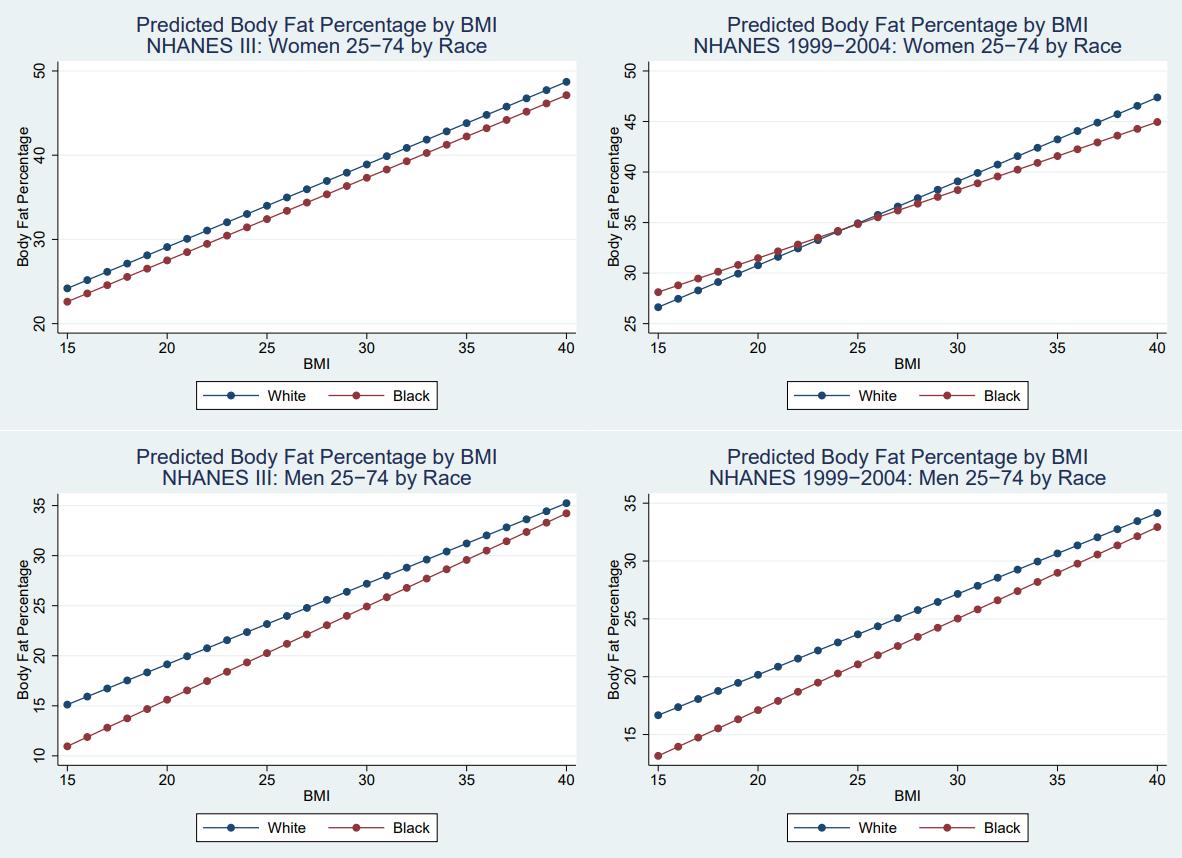
Figure 1, sourced from a 2008 study shows body fat plotted against BMI measurements categorized by both race and gender. The charts categorized as NHANES III present survey data from 1988-1994. The NHANES is the National Health and Nutritional Examination survey, which is a collection of cross-sectional studies performed by the CDC (Burke & Heiland, 2008).
Observing the chart on the top right, we see an intersection between the lines. This shows that for females with BMI values below around 24, Blacks are expected to report a higher percentage of body fat than their white counterparts (Burke & Heiland, 2008). This being the case, the opposite can be said when BMI levels surpass this amount (Burke & Heiland, 2008). In all the other supporting charts, we see that Whites are often predicted to report higher levels of body fat regardless of the level of BMI when compared to their black counterparts.
147
Source: NHANES III, NHANES 1999-2004 (Burke & Heiland, 2008)
Figure 2, sourced from a 2023 implications report presents a theoretical framework outlining the way in which structural racism links itself to physical and mental health complications within Black Americans. The theoretical model is included in this article to further stress the existence of an anti-Black sentiment surrounding the current systems controlling US healthcare. Within the original implications report, the current realm of empirical literature is discussed and critiqued (Reid & Earnshaw, 2023). The solid line within the model suggests a more concrete connection between two elements; in this case there is without a doubt a clear perceived relationship between the advent of structural racism and the onset of individual health issues in Black Americans. The dotted lines represent the less clear relationships; this is not to say that they are weak or non existent. Rather, literature and empirical studies need to evolve in order to more concretely describe the dynamics.
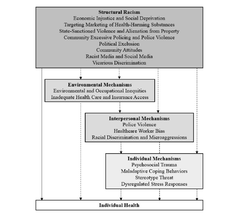
148
Source: Reid & Earnshaw, 2023 (adapted from Bailey et al., 2017)
LITERATURE REVIEW
The primary shortcoming of the existing research in this field is that it does not dive deep enough into both the economic factors and sociological/behavioral mechanics that work together to impact obesity rates. This being the case, several studies exist that offer luminous insights into both sides of the equation.
The aforementioned 2023 implications report offers a concise yet plenteous discussion on the current discriminatory sentiment disseminating across the US Healthcare system. Additionally, it also offers criticism that is intended to urge researchers to build upon longstanding limitations. The concept of structural stigma is introduced, and it is defined as a devaluating social process that works to “constrain the opportunities, resources, and well-being of the stigmatized” (Reid & Earnshaw, 2023). It is devaluating and socially demoralizing because it offers a lens towards how social phenomena can bleed into the values of institutions and cause concrete damage. The authors touch upon a 2001 study that attempted to identify the potential catalysts that resulted in segregated communities having worse levels of general health. The study found alarmingly intuitive results; exposure to toxins and inequities amongst access to quality health care were a few of the potential mechanisms found (Reid & Earnshaw, 2023).
The crux of the report is the inclusion of a model adapted from a 2017 study that attempts to find the pathways through which structural stigma can be linked to impacts on individual health. This is an essential model to understand because it offers visual evidence of the ways in which society’s mechanisms work to keep Black and other non-white individuals in a suppressed and demoralized state. It shows that everything is connected; the toolbox utilized by government officials during the redlining era is still being employed today. The only difference is that more and more tactics have been added to distort the reality that the primary way this system benefits is via the control of the non-white body, mind, and economic livelihood.
149
Using this theoretical framework as a foundation of sorts, attention can now be turned towards empirical studies that quantitatively attempt to highlight issues facing Black individuals regarding healthcare. A 2015 study analyzing statewide obesity prevalence offers an empirical model that attempts to identify what economic factors are most correlated to Black health issues (Broady & Meeks, 2015). The authors address the impact of the capitalist market on the obesity epidemic “fast food restaurant franchises are becoming more prevalent, consumers are buying more…obesity rates are increasing” (Broady & Meeks, 2015). There criticism is paramount; they argue that population detriments created as a result of support of the free market need to be checked by state and federal level policy changes (Broady & Meeks, 2015). National fitness initiatives, food accessibility programs, and general nutritional education. These are some areas that the authors feel a nation needs to place more of an emphasis, especially within the context of Blacks and their reported levels of health as a result of this lack of emphasis.
The model used within this report mixes a key number of lifestyle indicators and economic programs; SNAP benefit, physical exercise tendencies, and MRFEI (Modified Retail Food Environment Index) to name a few.
A 2008 study looked to address the discrepancies in obesity prevalence rates between Whites and non-whites using self reported survey data from the National Health and Nutrition Examination Surveys (Burke & Heiland, 2008). Within the data the study observed gaps in mean BMI and obesity prevalence between Black and white women (Burke & Heiland, 2008). This being the case, the gaps weren’t found to narrow significantly once things like education, income, and occupation were controlled for. The study concluded that black women face much weaker incentives to avoid becoming obese, and this is explained by a combination of both health related incentives and behavioral (Burke & Heiland, 2008).
A 2016 empirical work aimed to address the heightening level of public concern regarding health care costs by performing an analysis of the costs associated with obesity in the US. The study found that the annual level of spending on obesity related complications in 2014 was just under $150 million (Kim & Basu, 2016). 12 additional studies were gathered and observed within this report. Positive correlations were observed
150
between lifetime healthcare costs and rising BMI, which further suggests the reality that the condition leads to both financial and physical burdens (Kim & Basu 2016).
In 2019, researchers at FIU dove into an interesting potential relationship. They wanted to answer the question: is there any sort of correlation between violent crime and obesity rates? (Stolzenberg, D'Alessio, & Flexon, 2019). It is suggested that residing in a violent/unsafe neighborhood could potentially exacerbate obesity by pushing individuals to stay inside in order to avoid the dangers of their environment. The study observed data describing 12,645 residents living in 34 different NYC neighborhoods. It found that the probability of both a black and hispanic resident being obese increase additionally (Stolzenberg et al., 2019). Obesity and crime do not have a clear correlation; this study even noted that while increased probability of one led to an increase in the other, there wasn’t a direct link (Stolzenberg et al., 2019). The dynamic can be related to a plethora of factors; those who reside in poverty stricken areas probably will not have fair access to healthy food options. The study expounds upon this interesting dynamic and offers valuable insight into a correlation that is not often discussed in other literature.
A 2020 study within the Journal of Social Economics Research offers an empirical analysis of the differences in obesity trends between the East and Westt Coasts of the US (Adrangi, Hoppe, & Raffiee, 2020). To perform this analysis, the researcers built a model that captured food access and household income for both regions. To address food access, the model included metrics capturing the amount of grocery stores per country, fast food restaurants, and convenience stores. Recreational facilities per county was also included. The study concluded that policy recommendations stressing fast food corporations offering healthy options should be emphasized (Adrangi et al., 2020). Additionally, as the data showed a negative correlation with grocery stores and obesity, it is suggested that increasing access to these healthier food options would be a strong point for policies to fixate on (Adrangi et al., 2020). Of course these implementations are easier said than done.
This being the case however, this study serves as further justification that the capitalist drives of the franchise need to be examined if true public health reform it so be achieved.
151
DATA AND EMPIRICAL METHODOLOGY Data
The study uses cross-sectional statewide data from the year 2021. Data was obtained from a wide array of organizations and web databases. Data for the dependent variables of OBESITY_TOTAL, OBESITY_WHITE, and OBESITY_BLACK were sourced from the 2021 CDC web publication of statewide obesity prevalence. Data for the independent variable VIOLENT_CRIME was obtained from an online World Population Review database. Data for the remaining independent variables was sourced from Statista. Summary statistics for the data are provided in Table 1.
Table 1
Summary Statistics
Empirical Model
Following (Broady & Meeks, 2015) this study adapted and modified a model that was originally developed to determine the impact Supplemental Nutrition Assistance Program benefits (SNAP) and other lifestyle factors had on statewide obesity prevalence rates.
The original model is as follows:
Variable Obs Mean Std. dev. Min Max BLACK_PERC 51 0.1227451 0.1054908 0.01 0.47 FAST_FOOD 51 4894.078 5665.853 356 30867 HEALTH 50 8.6602 0.5562869 7.5 9.8 HOSPITAL 51 8.37E+07 1.06E+08 3444658 5.02E+08 INCOME 51 71532.88 11825.76 46637 97332 SNAP 51 799.7055 906.4409 29.83 4396.99 OBESITY_TOTAL 51 0.3193529 0.0400753 0.238 0.408 VIOLENT_CRIME 51 396.1042 175.9051 108.581 999.837 SMOKING 51 0.1294118 0.0294219 0.06 0.2 ALCOHOL 51 2.560196 0.5943955 1.36 4.83 GINITHEILINDEX 51 0.472549 0.0210564 0.43 0.54
152
This report adapts the model from the 2015 study and creates 2 separate models that attempt to capture the multifaceted indicators that have significant impacts on obesity rates for both Blacks and Whites. The first model attempts to recreate the findings of the first, while using some variables as a proxy. The variables SNAP and INCOME were pulled from the original model. As a proxy for LTPA, HEALTH was used. This was a selfreported score assessing the average level of physical well-being for the inhabitants of a given state. As a proxy for AFRICAN, BLACK_PERC was utilized. This variable captured the statewide percentage of Black inhabitants. In the original model, HEALTHY_FOOD was a quantitative variable that captured the percentage of census tracts that did not have at least one healthy food retailer (Broady & Meeks, 2015) MFREI was also utilized in the original model; it was the Modified Retail Food Environment Food Index. It measures the count of healthy and less healthy food retailers within a given census track. As a proxy for these variables, FAST_FOOD was utilized. This variable captured the total amount of fastfood restaurants in each state. The model adds in a measurement of inequality through GINITHEILINDEX. This measurement captured the average Gini coefficient estimate for each state.
The second model expounds upon the first by adding more explanatory models. The key variables appended to the model were ALCOHOL, HOSPITAL, SMOKING, and VIOLENT_CRIME. Both models set OBESITY_TOTAL as the key dependent variable. This was an estimate of the average levels of obesity prevalence for each state.
The models can be written as follows:
6MFRI+������������
1) β1SNAP + β2HEALTH + β3INCOME+ β4BLACK_PERC + β5FAST_FOOD + β6GINITHEILINDEX + ������������ 153
5.0 EMPIRICAL RESULTS
The empirical estimation results are presented in Table 2. The empirical estimation for the first model initially presents the negative relationship with SNAP and OBESITY_TOTAL. While the signage is appropriate, it is not a statistically significant finding. BLACK_PERC and FAST_FOOD both had a positive sign. This is appropriate, as the signage suggests that the higher the Black population in a state, the higher the prevalence of obesity is. This follows the findings of (Broady & Meeks, 2015). This was found to be statistically significant at a 5% level. INCOME and its relationship was found to be statistically significant at a 1% level. HEALTH, INCOME, and GINITHEILINDEX all had a negative sign. This follows the common perception most works of literature have surrounding these concepts; the more physically active someone is the less likely they are to succumb to a sedentary lifestyle/obesity. The more income an individual or household can acquire, the better quality of food they can purchase and the greater avoidance they have of obesity and its related ailments. The negative signage of the Gini coefficient variable suggests that as economic inequality increases, the prevalence of obesity seems to decrease. An increase in the Gini coefficient would suggest that the dispersion of income in each state has become more uneven. States with higher Gini coefficients are likely to have higher wealth and overall wellbeing. In regions with higher Gini coefficients, the disparity between affluent individuals and impoverished individuals is greater. This being the case, individuals with greater individual wealth can afford cleaner food, finance expensive exercise habits, and generally foster a lifestyle that extravagantly avoids a sedentary lifestyle. In both models, this coefficient is statistically significant at a 1% level. The R-squared for this model was 0.5232, which showed that the model was a good fit.

2) OBESITY_TOTAL
ALCOHOL
= β1
+ β2BLACK_PERC + β3FAST_FOOD + β4GINITHEILINDEX + β5HEALTH + β6HOSPITAL + β7INCOME + β8ASMOKING + β9SNAP + β10VIOLENT_CRIME + ������������
154
Table 2: Regression results OBESITY_TOTAL
Note: *** , **, and * denotes significance at the 1%, 5%, and 10% respectively.
In the second model, none of the key additional variables appended to the first were significant. The signages of the variables were appropriate. HOSPITAL represented the amount of revenue hospitals collected from patients statewide as a result of obesity related concerns. The positive sign supported the findings of (Kim & Basu, 2016) regarding rising healthcare costs and their impacts on obesity prevalence. The positive sign of smoking suggested that the more someone partakes in smoking, the more likely they were to find themselves susceptible to obesity and its related ailments. The adjusted R-squared for the second model was 0.5173.
I II CONSTANT .9154873*** .8320247*** SNAP -.0000128 -.0000147 HEALTH -.0217902*** -.0154657 INCOME -1.58e-06*** -1.22e-06 BLACK_PE RC .091163** .1026248** FAST_FOO D 1.22e-06 1.17e-06 GINITHEILI NDEX -.6366939*** -.636181*** ALCOHOL -.0100603 HOSPITAL 8.10e-12 SMOKING .232816 VIOLENT_C RIME -5.16e-06 R2 0.5232 0.5173 F-statistics 9.96 6.25 Number of obs. 50 50
155
CONCLUSION
In summary, the regression analyses included in this study suggest that there exists a significant level of anti-black discrimination within the U.S healthcare system. Additionally, it can be concluded that inequality - which was captured via the GINITHEILINDEX variable – serves as another significant influencer of the aforementioned healthcare discrimination. In terms of policy implications, legislation should place emphasis on improving the access that low SES census tracts have to clean and affordable food options.
Reflection on this study has led to the unearthing of key limitations that should be addressed if further replication is to be pursued. The first pertains to the data utilized within this study; the manual combination of multiple separate datasets to create one holistic data source could have resulted in some unwanted manipulation. If this study were to be revisited, it may be worthwhile to utilize more complete datasets, as the removal of the manual step of combining data - using programs like excel- could eliminate a certain level of human error. Another limitation was the fact that the study generalized statewide activity using data from an aggregate level. If the study utilized survey data, assessments could have been more individually focused. More individually focused assessments could have resulted in more variables being found significant. All things considered, this study expounds upon current literature within the field, and adds a fresh perspective that highlights key behavioral and economic factors that pertain to U.S healthcare discrimination.
156
Appendix A: Variable Description and Data Source
Acronym Description
Data source
OBESITY_TOTAL Statewide obesity prevalence in percentage. CDC
SNAP Supplemental Nutritional Assistance Program benefits allotted per person for each state
HEALTH 10 pt. score capturing individual well-being based on self-reported survey responses
STATISTA
STATISTA
INCOME Median household income for each state. STATISTA
BLACK_PERC Percentage of Black population for each state STATISTA
FAST_FOOD Number of fast-food retailers in given state STATISTA
GINITHEILINDEX Gini Coefficient for a given state. STATISTA
ALCOHOL Average consumption of alcoholic beverage in liters for a given state
STATISTA
HOSPITAL Amount of revenue collected by hospitals resulting from obesity related ailments/treatments
SMOKING Average consumption of cigarettes in packs per person for a given state
VIOLENT_CRIME Violent crime rate for a given state.
STATISTA
STATISTA
World Population Review
157
Appendix B- Variables and Expected Signs
Acronym
Supplemental Nutritional Assistance Program benefits allotted per person for each state
HEALTH 10 pt. score capturing individual well-being based on self-reported survey responses.
BLACK_PERC Percentage of Black population for each state
FAST_FOOD Number of fast-food retailers in given state
GINITHEILINDEX Gini Coefficient for a given state.
ALCOHOL Average consumption of alcoholic beverage in liters for a given state
HOSPITAL Amount of revenue collected by hospitals resulting from obesity related ailments/treatments
SMOKING Average consumption of cigarettes in packs per person for a given state
Variable
Expected sign
-
Description
SNAP
-
-
INCOME Median household income for each state.
+
+-
+
+
_
+ 158
Violent crime rate for a given state. + 159
VIOLENT_CRIME
Adrangi, B., Hoppe, A., & Raffiee, K. (2020). Socioeconomic Environment and Obesity on the US West and East Coasts. Journal of Social Economics Research, 107-117.
Bailey, Z., Krieger, N., Agenor, M., & Graves, J. (2017). Structural racism and health inequities in the USA: evidence and interventions. Lancet, 143-1463.
Broady, K. E., & Meeks, A. G. (2015). Obesity and Social Inequality in America. The Review of Black Political Economy, 201-209.
Burke, M. A., & Heiland, F. (2008). Race, Obesity, and the Puzzle of Gender Specificity. Boston: Federal Reserve Bank of Boston.
Kim, D. D., & Basu, A. (2016). Estimating the Medical Care Costs of Obesity in the United States: Systematic Review, Meta-Analysis, and Empirical Analysis. Value in Health, 602-613.
Reid, A. E., & Earnshaw, V. A. (2023). Embracing heterogeneity: Implications for research on stigma, discrimination, and African Americans' health. Social Science & Medicine.
Stolzenberg, L., D'Alessio, S. J., & Flexon, J. L. (2019). The Impact of Violent Crime on Obesity.
Miami: Department of Criminology and Criminal Justice, Florida International University.
BIBLIOGRAPHY
160
Empirical Analysis of Institutional Quality and Financial Development on Income Inequality in Central America.
Odette Mansour
Abstract:
This paper investigates the effect of Institutional Quality and financial development in middleincome in Central American Countries. The study incorporates information about how inequality in middle income has increased alarmingly and how we should consider improving the institution's quality. The outcomes show a positive relationship between Institutional Quality and financial development regarding middle-income society in Central American Countries, specifically: Panama, Costa Rica, El Salvador, and Honduras, which is why we suggested reforming institutional in Central American countries, letting international institutions such as the World Bank, United Nations, and IMF use their financial and political influences to promote strategies aimed at improving institutions, promote education, and create more employment in services.
JEL Classification: D31, D33, B52
Keywords: Institutional Quality, financial development, and Income inequality
a Department of Economics, Bryant University, 1150 Douglas Pike, Smithfield, RI02917.
Email: omansour@bryant.edu
161
The impact of financial development on income inequality has been inconclusive in the literature. Each dimension of financial development deputizes a different aspect and may have different impacts on income inequality. The role of institutional quality in moderating the impact of each dimension on income inequality is also dissimilar. This paper investigates the effect of Institutional Quality and financial development in middleincome Asian and Latin American Countries. The study incorporates information about how inequality in middle income has increased at an alarming level and how we should consider improving the institution's quality.
Some theory claims that financial development can reduce income inequality by helping the poor reach more opportunities to support the education for their children in the future (Galor & Moav 2004), reducing the fixed costs of gaining financial services for low-income individuals, enhancing welfare as well as boosting demand for lowskilled workers (Demirgüç-Kunt & Levine 2009), and giving the poor more financial access (Weychert 2020). However, other theories argue the opposite by stating that financial development can exacerbate income inequality since the rich are much easier and more advantageous for accessing financial institutions (Rajan & Zingales 2003), the poor gain little benefit when financial development rules to higher returns capital and higher payment for professionals in the financial sector (Greenwood & Jovanovic, 1990), and developed financial services expand the demand for high-skilled workers and their relative wages (Demirgüç-Kunt & Levine, 2009). This paper was guided by three research objectives that differ from other studies: First, Duc Hong Vo et al. (2019): This study was conducted to fill in this gap on two different samples for the period from 1960 to 2014: a full sample of 158 countries; and a sample of 86 middle-income countries. The findings from this study indicate that causality is found from economic growth to income inequality and vice versa in both samples of countries. Second, Mohan Ramesh et al (2017): Using seven alternative measures of the institutions, this study examines the impacts of the quality of institutions on poverty rates in developing countries. Third, Huynh et al (2022): This paper studies the effects of financial development with multidimensional analysis of two main categories (financial institutions and financial markets)
1. INTRODUCTION
162
and institutional quality on income inequality in 30 Asian countries in the period 2000 –2019.
The rest of the paper is organized as follows: Section 2 gives a brief literature review. Section 3 outlines the empirical model. Data and estimation methodology are discussed in section 4. Finally, section 5 presents and discusses the empirical results. This is followed by a conclusion in section 6.
2. INSTITUTION QUALITY AND FINANCIAL DEVELOPMENT
The graphs below show the two indicators of institutions' quality: control of corruption and the rule of law. We can observe how Honduras has a negative rule of law and, over the year, how the control of corruption is decreasing, which can explain why the value of the GINI coefficient (49.1, 48.2) in 2019-2020 in Honduras. Similar to Panama and El Salvador, both the rule of law and control of corruption hold negative values, which also explains the low value for the GINI coefficient. Costa Rica still has a low weight for their control of corruption and the rule of law; however, they are better than Panama, Honduras, and El Salvador.
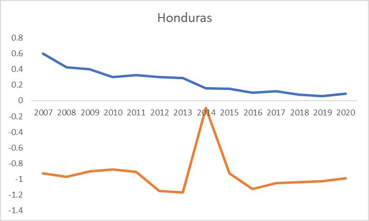
Institutional Quality Indicator in Honduras:
Source: WGI
Institutional Quality Indicator in Panama:
163
Source: WGI
Institutional Quality Indicator in Costa Rica:
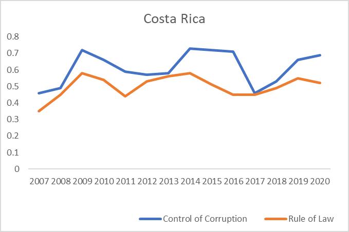
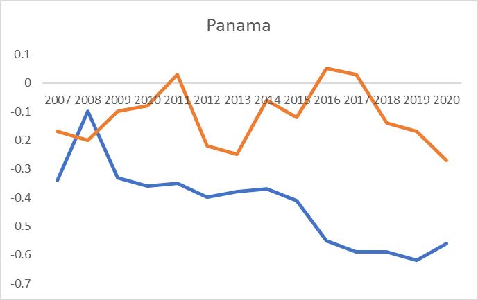
Source: WGI
Institutional Quality Indicator in El Salvador:
Source: WGI
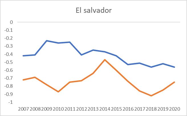
164
This study uses income inequality data from the World Development Indicators (WDI) and the world bank. For several countries, income inequality statistics are unavailable for all years, so we utilize the average poverty measures from 2007 to 2020.
In addition, we employ the financial development and institutional quality dimension to moderate the impact on income inequality.
3. LITERATURE REVIEW
A. The effect of financial development on income inequality:
The connection between financial development and income inequality is a topic of enduring controversy among economists. Some claim that financial development can decrease income inequality, others suggest it may aggravate it, and some argue that they hold an inverted U-shaped effect.
Firstly, financial development can improve access to credit and financial services, increasing economic opportunities and reducing income inequality. For example, it can help small businesses obtain funding, creating jobs and boosting economic growth. Additionally, financial development can facilitate the redistribution of wealth through government programs that use the financial system to transfer funds to lower-income households. Banerjee & Newman (1993) and Galor & Zeira (1993) theoretically present the negative effect of financial development on income inequality. They believe that financial development can reduce income inequality by supplying better credit availability that poor households can utilize for occupational alternatives to enhance their future income. Meanwhile, Galor & Zeira (1993) and Galor & Moav (2004) had different reasoning for the negative effect between income inequality and financial development through the channel of human capital investment that poor households earn from credits.
Clarke et al. (2006) empirically demonstrate that when financial development is more significant, income inequality becomes less in the long run for 83 countries between 1960 and 1996, as implied by Banerjee & Newman (1993) and Galor & Zeira (1993). The negative impact of financial development on income inequality is also due to boosting
165
demand for low-skilled workers and reducing the fixed costs of accessing financial services for low-income individuals (Demirgüç-Kunt & Levine, 2009). Weychert (2020) recently proved that financial access decreased income inequality in 52 countries from 2003 to 2014.
Secondly, financial development can also contribute to income inequality. It can help those who have already earned wealth by giving them more significant access to financial markets and investment opportunities. This can give them higher investment returns, broadening the income gap between the rich and the poor. Additionally, financial institutions may focus on serving wealthier clients, overlooking those with lower incomes and loosening their access to financial services. Accordingly, to Rajan & Zingales (2003), the wealthy get more advantages than the poor from financial markets since they are much more comfortable and more advantageous for accessing due to entry expenses. This broadens the income gap over time. In addition, Jauch & Watzka (2016) empirically found the positive effect of financial development on income inequality in 138 developed and developing countries from 1960 to 2008. Besides, De Haan and Sturm (2017) demonstrate that financial development and financial liberalization worsen income inequality for a sample of 121 countries during 1975-2005. Moreover, financial development increases income inequality since developed financial services increase the demand for high-skilled workers and their relative wages (Demirgüç-Kunt & Levine, 2009). Jaumotte et al. (2013) indicate that financial globalization is associated with growing income inequality in 51 countries from 1981 to 2003. This is demonstrated through the rising demand for skills and education, leading to a higher income. However, incomes disproportionately expand more for those who already have higher education and skills with high incomes.
Thirdly, Greenwood and Jovanovic (1990) theoretically present “the financial Kuznets curve”: income inequality increases at the initial phase because only the wealthy can afford to access and earn profit from financial markets, and falls after a certain level of economic development as the poor can join in financial markets with the progress in their incomes. Younsi and Bechtini (2018) illustrate that the financial development index increases income inequality and reduces it in the BRICS countries - Brazil, Russia, India, China, and South Africa between 1995-2015. Similarly, Azam and Raza (2018) show the
166
existence of such a financial Kuznets curve in ASEAN-5 countries, including Malaysia, Indonesia, Thailand, and the Philippines during 1989–2013- Financial development is measured by stock market capitalization, domestic credit to the private sector, and domestic credit by the banking sector. Nguyen et al. (2019) found similar results of an inverted U-shaped connection between financial development and income inequality for 21 emerging countries from 1961 to 2017. However, the study by Park and Shin (2017) reveals a U-shaped relationship between financial development and income inequality in 162 countries during 1960–2011: financial development reduces inequality up to the point of financial development, then beyond that, it worsens inequality. Those results conclude that the reducing-inequality effect of financial development becomes more effective in improved education and law order. Destek et al. (2020) found an inverted Ushaped relationship between income inequality and financial development proxied by overall financial development and banking sector development and a decreasing affinity between income inequality and stock market development in Turkey between 19902015.
Overall, the impact of financial development on income inequality is complex and may depend on the specific policies and institutions in place. Financial development can reduce income inequality by increasing economic opportunities and facilitating wealth redistribution. Still, it can also contribute to it by benefiting the already wealthy and neglecting the poor.
B. The impact of institutional quality on income inequality
Institutional quality can have a significant impact on income inequality. When institutions such as property rights, contract enforcement, and the rule of law are weak or ineffective, income inequality tends to be higher. This is because those with more power and resources can better control the system for their advantage, leaving less for those less well-off.
On the other hand, when institutional quality is high, income inequality manages to be lower. Emphatic institutions can ensure that everyone has access to the property and other resources and that contracts are executed fairly. This can form a more level playing field, allowing everyone to compete equally.
167
The vital role of institutional quality has been proved in the literature of various economic fields. Acemoglu et al., 2005, prove that income inequality not only drives economic development but also diminishes the harmful impact of climate change on economic growth (Hoang & Huynh, 2021). Institutional quality also enhances the beneficial impact of FDI on environmental quality (Huynh & Hoang, 2019) and moderates the impact of FDI on income inequality (Huynh, 2021). Especially it can lead to an equal income distribution because people experiencing poverty can be protected by an independent judicial system (Chong & Gradstein, 2007). Similarly, Carmignani (2009) proves that weak institutions lead to higher income inequality. Meanwhile, Gradstein et al. (2001) argue that the impact of democracy on inequality relies on ideology and political systems. They encounter that democratization substantially 9 decreases inequality in Judeo-Christian societies but not significantly in those of Confucian, Buddhist, and Hindu. Similarly, inequality is negatively impacted by democracy in countries with a parliamentary than a presidential system. Further studies also illustrate the negative consequence of institutional quality on regional income dissimilarities (Kyriacou & Roca-Sagalés, 2013; Ezcurra & Rodrìguez-Pose, 2014). In the current study, we demonstrate the negative impact of institutional quality on income inequality.
C. The joint effects of financial development and institutional quality on income inequality
There needs to research on the combined effect of financial development and institutional quality on income inequality. However, we enclose this simultaneous effect in our research for the following reasons. Substantial evidence suggests that financial development and institutional quality can significantly affect income inequality. Financial development directs to the degree to which a country's financial system can marshal and distribute resources efficiently. In contrast, institutional quality refers to the power and effectiveness of a country's institutions, including its legal and regulatory framework, governance structures, and property rights protections.
First, using the same variable for financial development (domestic credit to the private sector) to examine its effect on income inequality, Beck et al. (2007) find a
168
negative one while De Haan and Sturm (2017) show a positive one, implying that this impact may rely on another factor.
Second, this factor can be institutional quality as Velthoven et al. (2019) explain that income inequality induced by finance is associated with more income redistribution than inequality driven by other factors, implying that the inequality-increasing effect of finance can be redressed by policymakers who can affect various dimensions of institutional quality.
Third, better institutional quality encourages financial development via the rules of law, voice accountability, and government effectiveness (Khan H et al., 2020), and financial development reduces income inequality by giving the poor more financial access to improve their incomes (Beck at al., 2007; Weychert, 2020).
Fourth, if financial development improves income inequality, the progress in institutional quality helps facilitate this detrimental impact since better institutional quality provides better needs to protect people experiencing poverty (Chong & Gradstein, 2007).
Fifth, Le et al. (2020) also indicate financial development boosts income inequality. Still, this toxic effect reduces with the additional development of the financial system - primarily attributed to more satisfactory institutional quality (Khan MA et al., 2020).
Hence, we hypothesize that institutional quality can moderate the impact of financial development on income inequality.
4. DATA AND EMPIRICAL METHODOLOGY
A. Data
The study uses annual data from 2007 to 2020 for 4 countries in Central America: Costa Rica, El Salvador, Honduras, Panama. Data were obtained from the World. Development Indicators (WDI), and the world bank website. For several countries, the income inequality statistics are not available for all years, so we utilize the average poverty measures from 2007 to 2020. We utilize the financial development and institutional quality dimension to moderate the impact on income inequality. Summary statistics for the data are provided in Table 1.
169
Table 1: Regression Analysis
B. Empirical Model
Based on the theoretical background of Huynh, Cong Minh, and Tran, Hoai Nam (2022), previous studies, and the above arguments, we examine the impact of financial development and institutional quality and their relations to income inequality by operating the following panel data model. The model could be written as follow:
(1) GINI it = α0 + α1 FDit + α2 IQit + α3 FDit* IQit + α4 INF+ α5 Trade Openness + α6 EDU + α7 EMP + εit
i and t represent country and time, respectively; α1, α2, α 3, and βj are the respective coefficients; and εit is the residual term.
The dependent variable is income inequality (GINI), calculated by the GINI index from the Standardized World Income Inequality Database – SWIID (Frederick, 2020) GINI is "the estimate of Gini index of inequality in equivalized (square root scale) household market (post-tax and post-transfer) income, using Luxembourg Income Study data as the standard" (Frederick, 2020). With a more increased value indicating higher income inequality, this index delivers the best available country-level indicator of income inequality for international studies (Gimpelson & Treisman, 2018). This index has been employed in various prior studies, such as those by Afesorgbor & Mahadevan (2016), Le et al. (2020), and Lee et al. (2020)
Financial development (FD) and institutional quality (IQ) are the independent variables. FD is measured by two financial indicators in this research: the financial markets index and financial institutions depth (FID). Those two indicators are estimated numbers, ranking from 0 (lowest development) to 1 (highest development). The calculation for each indicator is described by Svirydzenka (2016). Using those two indicators will
Coefficients Standard Error t Stat P-value Lower 95%Upper 95%Lower 95.0%Upper 95.0% Intercept 9.74 11.500.850.40-13.4032.88-13.4032.88 EMP 0.45 0.076.850.00 0.310.58 0.31 0.58 Inflation -0.67 0.54-1.250.22-1.750.41-1.75 0.41 EDU 0.07 0.031.940.06 0.000.14 0.00 0.14 OPEN 0.16 0.062.890.01 0.050.27 0.05 0.27 Control of Corruption 5.48 5.960.920.36-6.5117.47-6.5117.47 Rule of Law -4.17 4.59-0.910.37-13.415.06-13.41 5.06 Financial Development Index 18.79 23.110.810.42-27.7065.28-27.7065.28 Financial Institutions Depth Index -39.23 31.30-1.250.22-102.2023.75-102.2023.75
170
provide a wider and more inclusive analysis of the influences of financial development with various dimensions on income inequality. This is a composite index of institutional quality captured in this research by two constituents: the Rule of Law and Control of Corruption. FD*IQ designates the relations between FD and IQ. Finally, X is a vector of control variables, including Trade openness (OPEN), Inflation (INF), Education (EDU), and Employment (EMP). The justification of these variables is given as follows: Trade openness: Trade openness can restrict income inequality (Borraz & Lopez-Cordova, 2007; Salimi et al., 2014) or can broaden it (Mahesh, 2016; Wong, 2016). We calculate trade openness by the import and export share in GDP collected from WDI (World Bank, 2020b). Inflation: Rising inflation rate can reduce income inequality by increasing the nominal income or decreasing the value of private debt (Rice & Lozada, 1983; Mocan, 1999; Heer & Maußner, 2005; Sun, 2011). Inflations also deteriorate relative income by reducing the purchasing power of people undergoing poverty (Siami-Namini & Hudson, 2019; Law & Soon, 2020). However, Balcilar et al. (2018) find a nonlinear effect of inflation on income inequality, i.e., inflation aggravates income inequality at a specific inflation threshold. Below this level, inflation reduces income inequality. In our study, inflation is calculated by the share of imports and exports in GDP, extracted from WDI (World Bank, 2020b).
Education: It is argued that education reduces income inequality by enhancing skill and income (Mincer, 1970; Gregorio & Lee, 2002; and O'neill, 1995). However, Battistón et al. (2014) controversy that the convexity of returns to 13 education leads to more income dispersion. Employment: Unemployment aggravates income inequality due to the falling income of society's poor and powerless groups. This destructive impact of unemployment on income inequality has been authorized by many scholars, such as Rice and Lozada (1983), Mocan (1999), Cysne (2009), and Sheng (2011). Hence, employment, especially in services, is a solution to reduce income inequality (Huynh & Nguyen, 2020). In the present study, we use employment in services from WDI (World Bank, 2020b) as an employment indicator. Due to the availability of all data in the empirical model (1), we collect them for four Central American countries in the period 2007 – 2020, including Panama, El Salvador, Costa Rica, and Honduras.
171
C. Empirical Results
The regression highlights interesting results as follows. First, the financial institution's development (FI) enhances income inequality while the Financial Institutions Depth Index worsens. The depth of financial institutions may harm people experiencing poverty due to the higher demand for high-skilled workers and their relative wages for comprehensive financial services, and the higher returns to capital and higher payment for professionals in economic sectors. In our research, we also demonstrate other determinants of income inequality in the context of Central American Asian countries, consisting of trade openness, inflation, education, and employment. On the one hand, education and career in services are found to reduce income inequality. The negative impact of education on income inequality supports the viewpoint that education helps reduce income inequality through improving skill and income (Mincer, 1970; Gregorio & Lee, 2002; and O'neill, 1995). Employment in services is also a tool to ease income inequality, supported by Sheng (2011) and Huynh & Nguyen (2020).
Trade openness and inflation may depreciate income inequality, and trade openness can widen disparities due to the challenging competition between skilled and unskilled laborers, as argued by Mahesh (2016) and Wong (2016). Meanwhile, the positive impact
Regression Statistics Multiple R 0.858899794 R Square 0.737708856 Adjusted R Square 0.693063555 Standard Error 6.490108569 Observations 56 Table 2: Regression Results df SS MS F Significance F Regression 8 5568.050316 696.006289 16.52377 2.54033E-11 Residual 47 1979.710934 42.1215092 Total 55 7547.76125
Table 3:
ANOVA
172
of inflation on income inequality is consistent with Siami-Namini & Hudson (20190 and Law & Soon (2020), with the standpoint that inflation can lower the purchasing power of people experiencing poverty. These results provide evidence that some institutions are more conducive to being affected by income inequality than others. Those results were consistent with the empirical analysis made by Huynh et al. (2022) that my research was primarily based on it.
5. CONCLUSION
The effect of financial development on income inequality has been imprecise in the literature, indicating that this result can be affected by other variables, and the outcome may depend on different dimensions of financial development. This paper examines the effects of financial development with a multi-dimensional analysis of one main category, the financial institutions and institutional quality, on income inequality in 4 American Central countries in the period 2007 – 2020. Results show that the financial institutions' development (FI), Control of Corruption, financial development index, and education reduce income inequality. Still, the financial institutions' depth index (FID), Open trade, and inflation increase it. In this sense, international institutions such as the World Bank, United Nations, and IMF could use their financial and political influences to promote strategies to improve institutions.
And institutions should be promoting education better while creating more employment in services.
173
APPENDIX
RESIDUAL OUTPUT
Observation Predicted GINI Residuals 1 48.20840143 1.091598566 2 47.69650947 0.903490531 3 48.32345984 2.276540164 4 50.85983101 -2.859831014 5 53.38257844 -4.582578444 6 53.16165245 -4.76165245 7 53.87537217 -4.675372171 8 52.98233517 -4.382335166 9 51.8677159 -3.467715895 10 53.7276771 -5.027677104 11 50.94923731 -2.649237305 12 51.50471579 -3.50471579 13 52.28087659 -4.08087659 14 20.70420569 28.59579431 15 42.69705889 2.502941108 16 42.14395694 4.756043056 17 44.50234712 1.297652876 18 43.57037572 -0.070375721 19 42.06699527 0.233004733 20 43.65033025 -1.850330252 21 45.91854525 -2.518545253 22 44.15190474 -2.551904743 23 38.34059513 2.259404868 24 38.57628201 1.423717991 25 38.69542625 -0.695426254 26 38.69299182 -0.092991824 27 38.92522943 -0.125229425 28 8.690646384 -8.690646384 29 54.83130176 0.968698244 30 53.40599756 2.094002436 31 42.80162587 8.498374126 32 51.13102466 1.968975345 33 51.5235896 1.0764104 34 53.91116402 -0.511164017 35 51.66908519 -1.66908519 36 43.45735502 6.442644976 37 46.45738437 2.742615625 174
38 48.33967933 1.46032067 39 46.78625146 2.61374854 40 48.74424908 0.155750916 41 46.43465607 1.765343934 42 19.06580996 -19.06580996 43 55.44349935 -2.743499347 44 56.54016885 -3.840168847 45 51.12254557 0.677454431 46 55.53549593 -3.935495932 47 55.35789639 -4.057896388 48 50.39639931 1.30360069 49 52.38271325 -0.882713248 50 49.45072804 1.049271957 51 48.89730069 1.902699314 52 45.78315927 4.61684073 53 45.35398232 4.546017677 54 42.32213 6.877869999 55 41.37599314 8.424006855 56 11.23156036 -11.23156036 175
BIBLIOGRAPHY
Huynh, Cong Minh, and Hoai Nam Tran. “Financial Development, Income Inequality and Institutional Quality: A Multi-Dimensional Analysis.” Munich Personal RePEc Archive, 22 Apr. 2022, https://mpra.ub.uni-muenchen.de/112829/.
Poverty, Geography and Institutional Path Dependence - LMU. https://mpra.ub.unimuenchen.de/10201/1/MPRA_paper_10201.pdf.
Vo, Duc Hong, et al. “What Factors Affect Income Inequality and Economic Growth in MiddleIncome Countries?” MDPI, Multidisciplinary Digital Publishing Institute, 8 Mar. 2019, https://www.mdpi.com/1911-8074/12/1/40/.
“World Development Indicators.” DataBank, https://databank.worldbank.org/reports.aspx?source=2&country=CRI.
“Data Catalog.” World Development Indicators, https://datacatalog.worldbank.org/search/dataset/0037712/World-Development-Indicators.
Ezcurra, R., & Rodrìguez-Pose, A. (2014). Government quality and spatial inequality: A crosscountry analysis. Environment Planning 46, 1732–1753.
Jung, S. M., & Cha, H. E. (2021). Financial development and income inequality: evidence from China. Journal of the Asia Pacific Economy 26(1), 73-95.
Khan, H., Khan , S., & Zuojun, F. (2020). Institutional Quality and Financial Development: Evidence from Developing and Emerging Economies. Global Business Review, 1-13. DOI: 10.1177/0972150919892366.
Law, C. H., & Soon, S. V. (2020). The impact of inflation on income inequality: the role of institutional quality. Applied Economics Letters, 1–4. doi:10.1080/13504851.2020.1717425
Park, K. H. (1996). Educational expansion and educational inequality on income distribution. Economics of Education Review 15 (1), 51–58.
Perera, L., & Lee, G. (2013). Have economic growth and institutional quality contributed to poverty and inequality reduction in Asia? Journal of Asian Economics 27, 71–86
Sheng, Y. (2011). Unemployment and Income Inequality: A Puzzling Finding from the US in 1941-2010. Available at SSRN: https://ssrn.com/abstract=2020744 or http://dx.doi.org/10.2139/ssrn.2020744.
176
Empirical Analysis of NBA Ticket Prices Correlation to NBA All-Stars
Michael McNeil
Abstract:
This paper investigates the possibility of a correlation between NBA ticket prices and if NBA All-Stars increase this cost. The model will incorporate the points, rebounds, assists, and minutes an NBA team has, the number of audience members, and how many All-Stars are at the game.
JEL Classification: L83, Z2
Keywords: NBA Allstar, Ticket Prices.
a Department of Economics, Bryant University, 1150 Douglas Pike, Smithfield, RI 02917. Email: mmcneil2@bryant.edu
177
1.0 INTRODUCTION
NBA ticket prices have increased a large amount over the last couple of years making it expensive for a fan to go to the game. Some reasons for this could be because of the inflation that has taken place and because of Covid. One question that I had while looking at these ticket price increases, is if this price increase could increase further if an All-Star is playing in the game. This thought came into mind because one of the features of the NBA that draw fans is the celebrity of many of the most famous players in the league.
This study aims to enhance understanding of why NBA tickets are so expensive and if one of the reasons is because of All-Star NBA players. To better understand this study, it will include many factors that go into why people choose to see an NBA game. This will include the team points, team wins, assists, NBA all-stars, and attendance. All these factors go into the regression because of the impact they potentially have on the overall price of NBA tickets. The largest impact on how enjoyable a game is for fans is the statistics that teams can put up during a game. When teams score many points in a game and keep it close for both teams, it will result in a more interesting game for the fans, leading to higher ticket prices. This also goes for the attendance of teams. If the game is more interesting, there is a higher demand for tickets, which would also result in higher prices. Lastly\, the reason for this study on NBA all-stars, there is a large lure to NBA all-stars that make a lot of people want to attend a game in person to watch these players play.
178
The research objective that guides this study is if NBA all-stars have a correlation to NBA tickets. While doing this study I will also be doing three regression analyses. The first is on NBA team statistics in the 2022 season with ticket prices, the second will be on team 2022 attendance with ticket prices. The last regression will be on NBA all-stars and ticket prices. These will all be evaluated and try to find if any of the variables will be correlated to ticket prices. The paper will be outlined as follows: Section 2 will be brief literature about 3 different studies on sports economics. Section 3 will be an outline of the empirical model that I used. Section 4 will be on the data estimation methodology. The discussion of the empirical results will be in section 5 and lastly, the conclusion will be in section 6.
2.0 NBA STATISTICS
Table 1: In the 2022 NBA season, each team played 82 regular-season games. The points earned by each team during these games were a crucial factor in determining their position in the standings leading to a team’s playoff seeding. NBA teams scored points through various methods such as field goals, three-pointers, and free throws. The top-scoring team in the 2022 season was the Minnesota Timberwolves, who averaged 115.9 points per game. The Memphis Grizzlies closely followed them, averaging 115.6 points per game. Other high-scoring teams included the Charlotte Hornets, Atlanta Hawks, and the Phoenix Suns. The points scored by each team contributed to the exciting competition and drama of the 2022 NBA season.
179
Table 1: 2022 NBA Team Statistics (Points)
Table 2: In the 2022 NBA season teams were able to play a total of 82 games in the season, this includes 41 of them being home games and another 41 being away games. Throughout that season, the team with the highest total attendance was the Chicago Bulls with 856,148 people, and the second was the Philadelphia 76ers with 846,867. Some other notable teams that totalled many fans were the Dallas Mavericks, Miami Heat, and the Boston Celtics. Other statistics that also went into attendance were the team’s average for home and away games as well as the team’s total for home and away games.
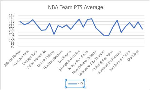 Source: ESPN
180
Table 2: NBA Team Attendance 2022
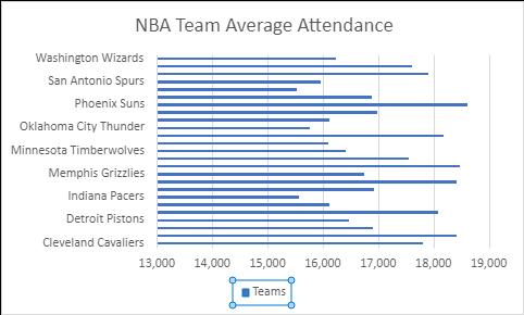
Source: ESPN
Table 3: The NBA All-Star Weekend is an annual event that highlights the league's top players from both the Eastern and Western Conferences. The All-Star Game provides an opportunity for fans to see their favourite players compete against each other in a highly competitive and entertaining setting. The players selected for the All-Star teams are chosen through a combination of fan, player, and media voting, with the most popular and skilled players earning spots on the rosters. Along with the game itself, the All-Star Weekend includes other events such as the Slam Dunk Contest, Three-Point Shootout, and Skills Challenge, which add to the excitement and entertainment value of the event. The NBA All-Star Game is considered one of the premier events of the basketball season, drawing fans from around the world and providing a platform for the league's top players to display their talents.
181
Number of NBA All-Stars Per Team 2022
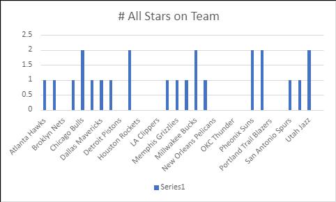
Source: ESPN
3.0 LITERATURE REVIEW
The study (Berri et al. 2004) examines the impact of star players on National Basketball Association gate revenues. The authors begin by introducing the concept of star power and its potential impact on ticket sales. They argue that star players have a significant effect on team performance, which in turn affects attendance and revenue. The authors conducted a study of the NBA from the 2002-2003 season through the 2006-2007 season, analyzing data on player salaries, team revenues, and ticket prices. They found that star players have a positive and statistically significant impact on gate revenues. The authors also found that teams with higher payrolls and more star players tend to have higher ticket prices. In addition to analyzing the impact of individual star players, the
182
authors also considered the impact of team-level star power. They found that teams with more star players, as measured by All-Star selections, tend to have higher gate revenues. Furthermore, they found that the impact of team-level star power is greater than the impact of individual star players. The authors conclude by discussing the implications of their findings for team management and player salaries. They argue that teams should invest in star players to increase gate revenues and that players should be compensated based on their impact on team performance and revenue (Berri et al. 2004). The authors also suggest that future research should explore the impact of star power on other aspects of team performance, such as merchandise sales and television ratings. Overall, Berri et al. provides compelling evidence of the impact of star power on NBA gate revenues. The study's findings have important implications for team management, player compensation, and future research in the field of sports economics.
Another study that investigates the relationship between ticket prices, concession prices, and attendance at professional sporting events is Coates and Humphreys (2007) study. The authors argue that understanding the impact of these factors on attendance is important for team management and policymakers’ decisions. The authors conducted a study of Major League Baseball (MLB) and National Football League (NFL) games from the 2006-2007 season. They analyzed data on ticket prices, concession prices, attendance, and other variables such as team winning percentage, market size, and stadium age. The authors found that higher ticket prices are associated with lower attendance, which is consistent with economic theory. However, the authors also found that higher concession prices are associated with higher attendance, which is counterintuitive. The authors suggest that this may be due to the "sunk cost" effect, where fans who have already paid
183
for expensive tickets are more likely to spend more money on concessions while attending the game. The authors also found that winning percentage and stadium age are significant factors affecting attendance, with winning percentage having a larger impact. Market size, however, did not have a significant effect on attendance. The authors conclude by discussing the implications of their findings for team management and policymakers. Coates and Humphrey suggest that teams should consider lowering ticket prices to increase attendance, but also be careful not to lower concession prices too much, as this may not have a significant impact on attendance but could lead to a decrease in revenue. They also suggest that policymakers should be aware of the impact of stadium age on attendance and consider investing in stadium renovations to increase attendance. Overall, (Coates and Humphreys 2007) provide valuable insights into the factors that affect attendance at professional sporting events. The study's findings have important implications for team management, policymakers, and future research in the field of sports economics.
In this research paper written by Scott D. Grimshaw and Jeffrey S. Larson (2021) that examines the impact of star players on television ratings for the NBA All-Star Game.
The authors argue that star players have a significant impact on the popularity of the AllStar Game and therefore on the ratings for the game's broadcast. The authors conducted a study of the NBA All-Star Game from 1991 to 2012, analyzing data on player salaries, player statistics, and television ratings. They found that the presence of star players, as measured by All-Star selections, and player statistics, has a positive and statistically significant impact on television ratings for the All-Star Game. The authors also found that the impact of star power on ratings is greater for games that are more competitive. In
184
addition to analyzing the impact of individual star players, the authors also considered the impact of team-level star power. They found that teams with more star players, as measured by All-Star selections, tend to have higher television ratings for the All-Star Game. Furthermore, they found that the impact of team-level star power is greater than the impact of individual star players. The authors conclude by discussing the implications of their findings for the NBA and its players. They argue that the NBA should continue to promote its star players and their participation in the All-Star Game to increase the game's popularity and television ratings. They also suggest that players should be compensated based on their impact on the league's revenue, including television ratings.
Overall, Star Power on NBA All-Star Game TV provides compelling evidence of the impact of star power on television ratings for the NBA All-Star Game. The study's findings have important implications for the NBA, its players, and future sports economics research.
In the study (Megia-Cayuela 2023) it explores the pricing strategy for tickets to first division teams in the Spanish soccer league during the 2018/2019 season. The way that they find their findings in this paper is by using a dual hybrid model with supply and demand and its relationship to the pricing of the tickets. In the paper they talk about multiple reasons that fans decide to attend these games. Some reasons include the game's atmosphere, level of the opposing team and the facility. All these things are put into thought when a fan decides to attend a game, they want to see a game that is good so they will look at the team's schedule and decide to attend a game against a good team. At this game fans will also be able to use the facility provided with concessions and clothing to buy while they are there. In the conclusion of the paper the findings were that the
185
difference in pricing for each club in the Spanish league was 300%. A second thing that was found as well was that only five out of the twenty clubs use the optimal pricing strategy when making up the ticket prices for the games.
The study (Steven Salaga and Jason Winfree 2015) explores the secondary market that has emerged in the National Football League with personal seat licenses (PSL) and season ticket rights (STR) sold electronically. With this data they were able to able to find out reasons for NFL ticket prices for games. In this study they were able to find that there was a correlation between both the price of tickets and the area in the stadium that you are sitting. If someone is sitting in the top of the stadium the ticket price for them will be cheaper than someone who is sitting much closer to the field. They also mentioned that there was a clear difference in STR and PSL markets with both having interest in NFL games and how a team is doing during a season having an effect on the market price for the tickets. Lastly, they were able to find that higher prices for an NFL ticket are associated with lower secondary market STR and PSL sales prices.
4.0 DATA AND EMPIRICAL METHODOLOGY 4.1 Data
The study uses cross-sectional data from the 2022 season of the NBA. Data were obtained from the NBA website to get the team averages in attendance, points, assists, rebounds, and much more. Other data was collected from ESPN to get the all-star information for that season. I was also able to collect data for team attendance during the 2022 season. I was able to get the average for home and away as well as the total for the season. Summary statistics for the data are provided in Table 1.
186
4.2 Empirical Model
Following Grimshaw and Larson (2021) this study adapted and modified from previous studies, they focused on how the NBA gains most of their viewers for the NBA All-Star game by getting celebrities to attend to make it more memorable for viewers. In their model, they focused more on television standpoints with viewers but had many of the same variables that I wanted to use in my module. One of the main differences was that they had player efficiency in their module, however, for this model I focused on team statistics instead.
I added team statistics, team attendance, and the number of all-stars per team to better understand
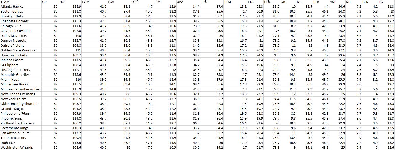
what variable affected
ticket prices. The model could be written as follow:
NBA Team Statistics 2022
Model - Ticket Prices = B0 + B1 AllStar + B2 PTS + B3 TO + B4 Team + B5 AST + B6 REB + B7 FTM + B8 FTA + B9 FT% + B10 HATT + B11 HAVG + B12 AATT + B13 AAVG Error Term 187
The first variable in my model is AllStar. This represents if each team has an NBA All-Stars on their team or not. This will be shown in the regression if a team has an AllStar on their team, it will count as a 1 and if they do not have any, it will be a 0. Within the model, there are the team statistics for the 2022 season, and these variables should allow teams to see if there was any correlation between team statistics and ticket prices. These variables include Points (PTS), Turnovers (TO), Assists (AST), Rebounds (REB), Field Throws Made (FTM), Field Throws Attempted (FTA), and Field Throw Percentage (FT%). The last variable is team attendance. This set of variables can influence ticket prices because if a team has more people attending games, then there is a higher demand for tickets which can result in a higher price. These variables include HATT (Home total attendance), HAVG (Home average attendance), AATT (Away average attendance), and AAVG (Away average attendance). The independent variable for this empirical module is the ticket price average for the 2022 season. These ticket prices are for each of the 30 teams in the NBA where they took the ticket prices for every game during the 2022 season and averaged them out.
5.0 EMPIRICAL RESULTS
The empirical estimation results are presented in Tables 2, 3, and 4. The empirical estimation shows a negative to no relationship for the first two regressions of Team Attendance as well as NBA All-Star. For the last regression though, it did show a positive relationship for some of the independent variables and NBA ticket prices. These variables were FTM, FTA, FT%, OR, DR, REB, AST, and TO.
188
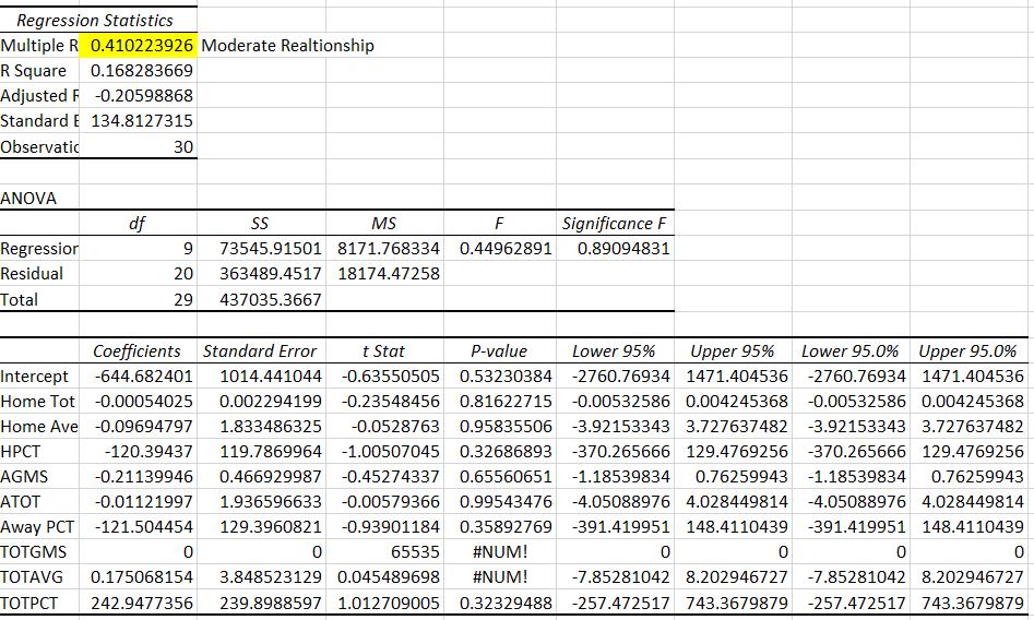
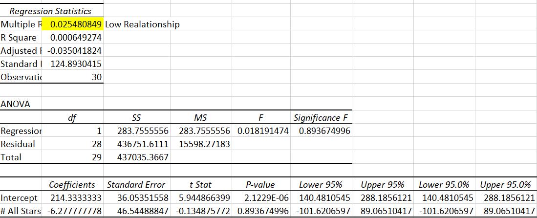 Table 2: Regression results for Team Attendance 2022
189
Table 3: Regression results for NBA All Star
The team statistics, as stated before, are shown to have a positive relationship because of the p-value that each of them has. This can be seen in Table 4 with the highlighted section for each independent variable. When looking at the table it is clear to see that each of the variable’s p-values are less than .05 meaning that they all have a positive relationship with ticket prices for NBA games. This finding can have a significant impact on teams that are trying to earn the most revenue during the season. Teams now can change the ways that they format their team in the future by adding larger centers and power forwards as well as more playmakers on teams to increase the statistics that have a positive relationship When a team adds more larger players to their roster, it helps teams get more rebounds on the offense and defense side of the ball. The reason for
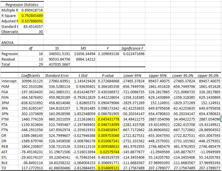 Table 4: Regression results for NBA Team Statistics 2022
190
this is that the height and size of these players will allow the team to get more rebounds much more easily. If a team also adds more playmakers, it will allow them to facilitate the ball which will allow for more shot attempts and assists. Moving the ball will also increase the chances of turnovers since it is less controlled. For tables 2 and three there was no correlation between All Stars and Attendance to ticket prices for NBA games. I was surprised to find that attendance for a team did not affect the ticket prices. The reason for this is because if a team has more fans attending a game, then it would not be surprising to see the ticket prices increase. If a team has more of a demand for tickets than to increase revenue, they would just increase the price of the tickets. Since there is a large demand, they will be bought no matter the price. I was also surprised to find that All Star players playing in the game had no relationship to the ticket price. I felt that people would be willing to pay more money to see these players in person, which would result in higher ticket prices.
5.0 CONCLUSION
In summary, NBA All-Star players do not have an impact on ticket prices for a team, but some team statistics do have an impact. These include FTM, FTA, FT%, OR, DR, REB, AST, and TO. Some of the limitations that come with my study include the inflation caused by the coronavirus. Since the virus did not allow people to be in close contact with each other this caused all teams to not allow fans to attend games. This could have affected how teams priced their tickets since they were trying to make up for the profits lost during the virus. If an NBA team wants to increase its revenue throughout its season, then it will want to increase these statistics. If a team wants to do this, they will need to build their rosters in a way that will allow them to be a winning team and
191
increase these statistics. Teams will need to add more centers and power forwards to their teams to increase rebounds and playmaking. Adding more centers and power forwards will allow teams to increase the number of rebounds they can get on the offense and defense side of the ball. Centers and power forwards are larger players in NBA and focus their attention on the court at the paint which is the closest to the basket. Since they play around there for their teams it means that they have a higher chance of getting rebounds. Playmakers in the NBA play either the point guard or shooting guard position, their main objective while playing is to create space and shot attempts for teammates by passing the ball and getting by on their defender. Getting their teammates open and shooting the ball themselves it will allow for more FTM, FTA, and FT%. Passing the ball is also sometimes dangerous to teams because it could lead to turnovers if a player is not paying attention or makes a risky pass. These findings I found from my empirical analysis do not line up with the findings I found from (Coates and Humphreyes 2007), (Berri et al 2004) and (Grimshaw and Larson 2021). In those findings they were able to find that revenue for teams were based off if a celebrity was at the game and the concession stands had an effect. One of the ways I could have had my results line up with previous studies is by adding a section of how many celebrities attended games for teams. This would allow for me to see if adding celebrities to games has any effect on the price of tickets to a game.
If an NBA team wants to increase ticket prices for games, they will need to increase FTM, FTA, FT%, OR, DR, REB, AST, and TO make the most revenue within a season.
192
BIBLIOGRAPHY
Coates, Dennis, and Brad R Humphreyes. “Ticket Prices, Concessions and Attendance at Professional Sporting Events.”
Https://Itservices.cas.unt.edu/~Jhauge/Teaching/Sports/monopoly_Coates_Humphreys_20 07.Pdf, International Journal of Sports Economics, 2007, https://itservices.cas.unt.edu/~jhauge/Teaching/Sports/monopoly_Coates_Humphreys_200 7.pdf.
Berri, David, et al. “Stars at the Gate: The Impact of Star Power on NBA Gate Revenues.” ResearchGate, Journal of Sports Economics, Feb. 2004, https://www.researchgate.net/publication/247739515_Stars_at_the_Gate_The_Impact_of_ Star_Power_on_NBA_Gate_Revenues.
Grimshaw, Scott D., and Jeffrey S. Larson. “Effect of Star Power on NBA All-Star Game TV Audience.” Journal of Sports Economics, vol. 22, no. 2, Feb. 2021, pp. 139–63. EBSCOhost, https://doi.org/http://jse.sagepub.com/content/by/year.
Megia-Cayuela, Daniel. “Valuation of Ticket Prices for First-Division Football Matches in the Spanish League.” Managerial and Decision Economics, vol. 44, no. 1, Jan. 2023, pp. 576–94.EBSCOhost,search.ebscohost.com/login.aspx direct=true&db=ecn&AN=2032460&site=ehost-live.
Salaga, Steven, and Jason A. Winfree. “Determinants of Secondary Market Sales Prices for National Football League Personal Seat Licenses and Season Ticket Rights.” Journal of Sports Economics, vol. 16, no. 3, Apr. 2015, pp. 227–53. EBSCOhost, https://doi.org/http://jse.sagepub.com/content/by/year.
193
Empirical Analysis of NFL Ticket Price Determinants
Kenny Page
Abstract:
This research paper examines the determinants of revenue for National Football League (NFL) franchises with respect to ticket prices. Using a dataset of ticket prices and various factors such as team performance, stadium capacity, market size, and team revenue, we analyze the relationship between ticket prices and a franchise’s revenue. The results align with past studies in this area of research as they indicate that past team performance and average attendance have the strongest effect on ticket prices. Additionally, the results reveal that stadium capacity and market size most significantly affect team revenue. We find that ticket prices are less sensitive to stadium capacity and market size than team performance. Again, the results align with previous literature as the findings suggest that teams price their tickets corresponding to the inelastic portion of demand. Overall, this study provides insights into the economics of NFL ticket pricing and highlights the importance of strategic decision-making in maximizing revenue for teams.
JEL Classifications: Z23,
Keywords: Sports Economics, Profit Maximization, Price Elasticity of Demand
Department of Economics, Bryant University, 1150 Douglas Pike, Smithfield, RI 02917
Phone (203) 999-9985. Email: Kpage3@bryant.edu
194
1.0 Introduction
Prior to the 2022 season, Forbes.com evaluated every NFL team as being worth at least over $3 billion. This past year, the valuation for the average NFL team increased 28% to $4.47 billion. A major aspect of the NFL’s revenue stream is ticket sales, which contribute significantly to a team’s financial success. There are several economic factors that contribute to the complex process of NFL ticket pricing.
From the Forbes valuations stated previously, the NFL has been consistently found as the most profitable league in the United States. Despite popular criticism laid out on owners for charging so much out of pure greed, sports economists generally find that fans actually pay a lower price than that which would maximize profits for the team. In sports economics, ticket prices are commonly assumed to correspond to the inelastic portion of demand, which is below the profit-maximizing price of an NFL team. Understandably, the reoccurring findings of inelastic ticket prices below the profit-maximizing level raise questions for researchers, and there are few explanations for this behavior.
This research paper aims to analyze NFL ticket price determinants by focusing on the factors which impact prices the greatest. Using a dataset of average ticket prices and numerous economic factors such as regional population, stadium capacity, team revenue, and average attendance, this study attempts to examine the factors that most affect NFL franchise revenue and their corresponding ticket prices. These factors are also complemented by “variables of prestige” such as win percentage, number of pro bowlers, and number of Super Bowl wins as of the 2022 season. By testing these variables against the dependent variables (average ticket prices and team total revenue) the study can identify possible relationships between the listed factors and NFL ticket prices.
The paper is organized so we first provide an overview of the relevant literature on the economics of professional sports as well as the factors that influence ticket prices. Then, we will describe the strategy and methodology for gathering and testing the data, including the variables and statistical methods. To conclude, we will next present the results of the analysis and discuss the implications of the findings for teams and their fans.
195
The findings in this study contribute to the understanding of the economics of the NFL while providing insights into the factors determining ticket prices. By identifying the key determinants, this study may help NFL teams make strategic decisions about ticket pricing and optimize their revenue streams. The research has valuable implications for fans just as much for teams, as fans may use the findings in this study to shed light on the factors that influence the cost of attending their favorite football team’s game.
2.0 Price Elasticity of Demand for NFL Ticket Pricing with Respect to Revenue
The accepted reasoning for this inelastic ticket model is related to profit maximization when other non-ticket revenues are included in the team’s objective plan. In this theory, owners follow additional multiproduct to their pricing strategy. Ticket prices in this theory are set in the inelastic region of demand to maximize total stadium revenues which includes parking, concessions, merchandise, etc. (Krautmann and Berri, 2007). Similarly, other researchers with this theory often include local and shared television revenues as trade-offs to inelastic ticket pricing (Brunkhorst and Fenn, 2010). Figure 1, it is listed as the top twelve most expensive NFL games to attend.
Rank Team Average Ticket 16oz. Beer Hot Dog Parking Total 1. Las Vegas Raiders $153.47 $12 $8 $100 $273.47 2. San Francisco 49ers $139.71 $11.50 $5.50 $85 $241.71 3. New England Patriots $131.45 $8.40 $4.50 $80 $224.35 4. Dallas Cowboys $99.50 $9.50 $6 $95 $210 5. Carolina Panthers $114.67 $10.50 $3 $81 $209.17 6. Los Angeles Rams $103.62 $13.75 $8 $80 $205.37 7. Washington Commanders $110.07 $11 $5 $65 $191.07 8. Philadelphia Eagles $127.06 $14.67 $6 $40 $187.73 9. Green Bay Packers $128.93 $9.50 $6 $40 $184.43 10. Los Angeles Chargers $80.38 $13.75 $8 $80 $182.13 11. Baltimore Ravens $110.38 $8.13 $3 $55 $176.51 12. New York Giants $115.31 $13 $7 $40 $175.31
Figure 1: Inelastic Pricing of NFL Tickets (Top 12 most expensive games to attend)
196
Source: James Brinsford; Newsweek
There is an abundance of literature that covers studies on a professional team’s attendance, revenue, and individual ticket pricing. Many of them focus on gate receipts alone, while others focus primarily on secondary ticket transactions from third-party sellers (Salaga and Winfree, 2013; Diehl et al., 2015). As well, a few (Marburger, 1997) model sports teams as multi-product monopolists that sell both admission and concessions. There are other arms of this type of literature that focus on the relationship between ticket prices and home-field advantages. This study, however, will be focusing on the average ticket price (average of both gate receipt and secondary market) for a specific team throughout the duration of a given season concerning prestige variables such as the number of star players and Super Bowls won by a given franchise.
In this area of study, it is a challenge to obtain price and quantity data for variables that pertain to individual teams such as quantity demanded, seat quality, and ticket complements, especially since all stadiums do have capacity restrictions. As a result, researchers have heavily relied on aggregate demand attendance figures and average ticket prices which are impossible to capture the true variation in demand that exists for specific seating locations, and accordingly the consumer types (Marburger, 1997; Fort, 2004; Diehl et al., 2015). Furthermore, total attendance measurements do not provide information on the number of spectators in a particular section, or a particular type of ticket. To clarify, it is difficult to distinguish whether a certain ticket holder owns season passes or is simply a single-game ticket holder. Given the countless amounts of seats and sections for the stadiums examined, such price averages are likely to be biased estimators of the prices paid by ticket holders. Therefore, it is also likely that the average price given in this field of study understates the price of the most desirable tickets (lower-level and box seats), and consequently overstates the average price of the least desirable tickets (upperlevel seating). It is also important to note that more desirable tickets are more likely to be sold out compared to less desirable tickets (Krautmann and Berri, 2007; Diehl et al., 2015). Figure 2 displays the top 24 teams based on average home attendance for the 2022 season. Through Figure 2, one may receive a better understanding of the team’s market size, it is no surprise that Dallas and the two New York teams are the top three by average attendance. However, being that Green Bay is a relatively smaller market size, it is surprising to see the Packers rank fourth, yet their fan base is famously known for being one of the most loyal in sports.
197
Another variable in this field of study that is considered valuable, yet hard to obtain, is fan loyalty. The most loyal customers of a sports franchise are their season ticket holders, who are generally considered to be less sensitive to ticket price year-over-year changes. In previous research, it has also been consistently found that single-game buyers have a greater price elasticity than season ticket holders, accordingly, single-game buyers are classified as casual fans (Scully, 1989: Simmons, 1996; Fort, 2004; Diehl et al., 2015). For this study, the geographic population for each team has been obtained in the hope of finding a correlation between ticket prices and the population of the region in which a team is located. In this sense, this element is brought into the study for teams such as the Green Bay Packers and the Buffalo Bills. The regional population must be utilized in this field of research so that the fan loyalty variable can
Rank Team Games Total Average Percentage 1. Cowboys 9 841,192 93,465 93.5 2. Jets 8 624,075 78,009 94.6 3. Giants 9 688,266 76,474 92.7 4. Packers 9 685,623 76,180 96.5 5. Broncos 8 607,845 75,980 99.8 6. Chiefs 8 587,997 73,499 100.8 7. Rams 9 654,606 72,734 101.7 8. 49ers 9 644,661 71,629 104.6 9. Panthers 9 642,167 71,351 96.7 10. Ravens 8 564,714 70,589 99.8 11. Chargers 8 559,644 69,955 97.8 12. Eagles 9 628,828 69,869 100.0 13. Falcons 9 626,248 69,583 92.8 14. Buccaneers 9 620,898 68,988 103.2 15. Saints 9 620,889 68,987 96.1 16. Seahawks 9 619,491 68,832 100.1 17. Titans 8 548,929 68,616 99.2 18. Bills 8 547,450 68,431 95.5 19. Texans 8 543,294 67,911 94.3 20. Browns 8 539,448 67,431 100.0 21. Vikings 9 600,183 66,687 100.3 22. Jaguars 8 531,675 66,459 97.9 23. Steelers 8 530,243 66,280 96.9 24. Bengals 7 463,733 66,247 101.1
Figure 2: Average Home Attendance (Top 24 franchises based on home attendance)
Source: ESPN.com
198
be potentially tested. It is known that Buffalo and Green Bay have some of the most passionate fans in the NFL while being in lesser populated regions compared to markets like Los Angeles or New York.
3.0 Literature Review for NFL Ticket Pricing
NFL teams face a variety of costs associated with operating their franchises. These costs contain player salaries, stadium expenses, marketing costs, and other operating costs that are necessary for the franchise. To combat these costs, owners use a variety of strategies to generate profits including pricing strategies, revenue sharing, and licensing agreements. Understanding these strategies and their impact on profit maximization is important for both team executives and fans (Brunkhorst and Fenn, 2010). In Brunkhorst and Fenn’s study, the two men conducted a study examining the factors affecting profit maximization in the NFL. In their study, the men were able to gather data on revenue, costs, and profits for 32 NFL teams during the 2007 NFL season. The analysis focused on two main strategies: ticket pricing and revenue sharing. Ticket pricing was found to be a significant factor in profit maximization. Brunkhorst and Fenn (2010) found that teams that charged higher prices for tickets tended to achieve higher profits. Accordingly, the two men also found that the teams who charged the highest prices also tended to have lower attendance rates, suggesting a possible trade-off between ticket prices and attendance. The other main strategy analyzed, revenue sharing, was also found to be a significant factor in profit maximization. In the NFL, there is a revenue-sharing system in which all teams share a portion of their revenue, including revenue from ticket sales, merchandise, and broadcasting rights. Brunkhorst and Fenn (2010), find that revenue sharing has a positive impact on profits for smaller-market teams, but a negative impact on profits for larger-market teams. Their conclusion suggests that revenue sharing may help level the playing field for small-market teams yet have unintended consequences for larger-market teams. The two men also call for the exploration of further research on how these two main strategies may vary across different markets over time.
While there is a substantial amount of research and data on the topic of professional sporting event ticket prices, there is a lack of literature on the NFL specifically. Salaga and Winfree (2013) looked to find the determinants of NFL ticket prices. In their study, they were cleverly able to obtain a gauge of these determinants by testing the resale price of individual
199
teams’ Personal Seat Licenses (PSLs) or Season Ticket Rights (STRs) in the secondary resale market. In Salaga and Winfree’s article, the two researchers view PSLs and STRs as an excellent way for NFL franchises to generate revenue. However, when fans buy these PSLs and STRs, they are very easily able to sell single-game tickets on the secondary market. Salaga and Winfree viewed the secondary market as a better determinant of ticket sales as there is more of an element of pure supply and demand. The data examined was on PSL and STR sales prices for all 32 NFL teams during the 2011 season. A variety of other factors such as stadium characteristics, team performance, and market demographic were also tested. Salaga and Winfree concluded that all three of these factors are statistically significant to secondary market prices. Tickets for teams with higher winning percentages, teams with newer and more comfortable stadiums (and higher capacity stadiums), and teams with fans of greater population size and income levels are found to have significantly more expensive secondary market ticket prices.
Pricing strategies in professional sports are complex with many factors influencing the price of tickets and concessions. While there are many studies on the factors determining ticket prices of professional franchises, Krautmann and Berri’s (2007) study aimed to investigate the price elasticity of demand in the context of concession pricing in professional sports. To measure the price sensitivity of fans, Krautmann and Berri gathered data on concession prices and sales volume for Major League Baseball, the National Football League, the National Basketball Association, and the National Hockey League during the 2004-2005 seasons. The study found that the price elasticity of demand for concessions varied depending on the league and the type of concession. For example, beer and hot dog sales were found to be relatively inelastic in the NBA and MLB, while being relatively elastic in the NFL. Over the big four professional leagues, the study found that the concessions with higher prices tend to have lower sales volumes, indicating that fans are generally price-sensitive when it comes to concessions. The study is also consistent with future findings on ticket prices as the teams with the highest quality rosters and opponents positively influence the price elasticity of demand (Krautmann and Berri, 2007).
The secondary market for sports tickets has become a crucial source of revenue for many professional sports teams. For franchises to maximize profits, NFL team executives must understand the price elasticity of demand for these tickets. Diehl et al. (2015), performed a study on this topic to investigate the sensitivity of consumers to changes in ticket prices. In this study,
200
the three researchers use data from the NFL to shed light on this NFL fan price sensitivity. In the context of sports tickets, understanding the price elasticity of demand allows franchises to maximize revenues by setting prices that will maximize profits while also attracting the maximum number of fans. Diehl et al. (2015) focused their analysis on the price elasticity of demand for regular season games, playoff games, and the Super Bowl. The results from their study suggest that NFL fans are relatively price-sensitive to game tickets in the secondary market, particularly for higher-demand events such as the Super Bowl. Other factors such as team performance, stadium capacity, and market demographic were found to be significant predictors of demand in the secondary market. The findings by Diehl et al. (2015) align with previous studies (Krautmann and Berri, 2007) as team performance, stadium capacity, and market size were all positively correlated with higher demand for tickets in the secondary market.
In another attempt to capture evidence of the price elasticity of demand in professional sports, Coates and Humphreys (2007) examined the relationship between ticket prices, concessions, and attendance at all major four professional sporting events in their study. Like the other study performed by Krautmann and Berri (2007), Coates and Humphrey also collected data from the MLB, NBA, NFL, and NHL, but during the 2002-2003 seasons. However, unlike Krautmann and Berri, Coates and Humphery focused their study on the effects of ticket price changes rather than concession stands. Coates and Humphrey (2007) found that higher ticket prices were typically associated with lower attendance, especially for weekday games. As well, the two men found that the effect of ticket prices on attendance varied depending on the quality of the team and the importance of the game. To clarify, higher ticket prices were found to have a smaller negative impact on attendance when the game means more, such as a playoff game or a game between two teams with winning records.
Professional sports franchises are often accepted as drivers of local economic growth and development. Yet, just as often city councils reject the idea of hosting professional teams, therefore making it a subject of debate of just how beneficial it is to host a professional sports team in one’s local community. Kuznitz (2011) examines the local economic impact of the four major professional sports leagues and their teams in the United States in his study. In the study, Kuznitz classifies the economic impact of professional teams into two categories: direct and
201
indirect. The direct impact includes the spending by teams on goods and services within the local economy, while the indirect impact includes the economic activity generated by fans attending the games, such as spending on hotels and community restaurants. Kuznitz (2011) found that the economic impact of sports teams on their local economy is often overstated. The study finds that the direct impact of teams on the local economy can be substantial, however, the indirect impact is often minimal. These findings are especially apparent with teams that have low-performance records and poor-quality rosters. Furthermore, many of the economic benefits of sports teams, such as job creation and new infrastructure, are generally temporary and often do not lead to long-term economic growth (Kuznitz, 2011).
4.0 Data and Empirical Methodology
4.1 Data
The study utilizes 2021-2022 cross-sectional data for the variables potentially affecting NFL team revenue and ticket prices. The data used in this study are derived from multiple sources. 2022 NFL team revenue was found from Forbes valuations, 2021 average price per ticket, amount of Super Bowl wins, and the number of teams per region was found from Statista.com. The study also used data on the 2021-win percentage, 2022 average attendance, 2022 returning Pro Bowlers per team, and team stadium capacity from ESPN.com. Finally, the last variable, region population (market size), was attained from census.gov. Summary statistics for all variables are listed in Tables 1 and 2.
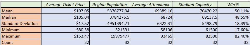 Table 1: Summary Statistics
202
Table 2: Summary Statistics
4.2 Empirical Methodology
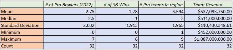
The model that is adopted and modified in this study is acquired from Brunkhorst and Fenn’s (2010) study. From their study, this study can embrace specific variables such as home attendance, winning percentage, the population of the home city, Pro Bowl selections, stadium capacity, and dummy variables for divisions. This study differs from Brunkhorst and Fenn’s, as this tests for revenue concerning ticket prices, rather than profit concerning ticket prices. Moreover, here tests for revenue rather than profit due to the lack of sufficient 2022 data on player, stadium, and team operational expenses. In these models, we have added the 2022 average ticket per home team, total revenue for each NFL team, the number of Super Bowl wins a franchise has achieved, and the number of pro teams within the NFL team’s region. We introduced Super Bowl wins and the number of pro teams within region variables as this study hypothesizes that these factors play a significant role in an NFL team’s revenue and ticket prices.
In this study, three separate models were used to display changes in an NFL team’s revenue and average ticket price. The models can be written as follows:
The first two models that are tested in the study pertain to the determinants of an NFL team’s total revenue. This is the first dependent variable that is examined as it is viewed that team revenue is a better measure of fans actual choices (Krautmann and Berri, 2003; Salaga and Winfree, 2013; Diehl et al., 2015) than simply average ticket price TRt represents the total revenue of a specific NFL team t, at the beginning of the 2022 regular season. Data on all 32 teams’ total revenue was found from Forbes’ 2022 NFL valuation rankings. From the rankings, notably, the Dallas Cowboys experience the highest revenue with $1.087 billion, while the
������������ = ������������ + ����1 ���������������� + ����2 ���������������� + ����3 ���������������� + ����4 ���������������� + ����5 ����%���� + �������� (Model I) ������������ = ������������ + ����1 ���������������� + ����2 ���������������� + ����3 ���������������� + ����4 ���������������� + ����5 ����%���� + ����6 �������������������� + ����7 ������������ + ����8 ���������������� + �������� (Model II)
203
Detroit Lions experience the lowest NFL revenue at $452 million. In this study, Diehl et al. (2015) definition of revenue is used as this study also assumes that tickets are priced in the inelastic portion of demand, meaning that franchises price tickets at a level lower than the profitmaximizing price. Therefore, for this study, we view the NFL team’s revenue as the total gate receipts divided by the total attendance, plus non-ticket stadium revenues such as parking, merchandising, and concession sales (Diehl et al., 2015; Depken, 2001; Scully, 1989).
There are seven independent variables used to investigate the determinants of total team revenue. Appendix A provides the acronyms, descriptions, and data sources for each variable used in the study. First, Popt (the regional population of the home city t) represents the market size of a specific team. Variable #2 is Attt, which simply represents the average attendance throughout the 2022 season for NFL team t. Followed by Capt, the total stadium capacity of team t. The study also uses PTRt, representing the amount of other professional sports teams located within the same state or region as team t, whether the team is in the NFL or any of the other three major North American professional leagues. This study also introduces “variables of prestige”. The first prestige variable is W%t, which is the specific 2021 season winning percentage of team t. The next variable of prestige utilized was ProB1, which is the number of Pro Bowlers expected to play on team t’s roster in the 2022 season, this variable displays the number of all-stars a team has on its roster. The final prestige variable is SBt, this is considered the main variable of prestige as it represents Super Bowl championship titles, which is something not every NFL team has attained and is a variable that is often neglected in this area of research.
The last model that is tested in the study pertains directly to a specific NFL team’s average ticket price. ATPt represents the average ticket price of a specific team, t. Unlike TRt, ATPt does not have a definition to it as it is simply the average of all gate receipt and secondary market prices taken at the end of the 2021 season. The data on average ticket prices derive from Alan Snel’s, from LVSportsBiz.com, “fan cost index” which ranks Las Vegas Raider tickets most expensive at $153.47 and ranks Las Angeles Chargers tickets the least expensive at $80.38. Because this study does not consider other costs for fans associated with ticket prices such as costs for parking, concessions, and merchandising, this study only includes the average ticket
���������������� = ������������ + ����1 ���������������� + ����2 ���������������� + ����3 ������������3 + ����4 ����%���� + ����5 ������������ + ����6 �������������������� + ����7 ������������ + ����8 ���������������� + �������� (Model III)
204
price index rather than the combination of average ticket price and fan cost index that is found in Coates and Humphreys (2013) study.
Like the models that we ran to investigate total team revenue, we use the same blueprints to test average ticket prices. Utilizing the same six independent variables as in models I and II, team total revenue is added into the regression for average ticket prices.
5.0 Empirical Results
Presented below are the empirical results from regression models I, II, and III. Model II has the best fit out of all the regressions run, accounting for 73% of the variation in the dependent variable Team Revenue. Model I also fit well explaining 67% of the variation in the dependent Team Revenue variable. In both models, I and II, the independent variables Average Attendance and Stadium Capacity are significant at a 1% level However, these models do differ somewhat. In Model I, Average Ticket Price is statistically significant at the 5% level Furthermore, model II displays that Regional Population and Super Bowl titles are both statistically significant, Super Bowl wins being more significant to Team Revenue than Regional Population. Average Ticket Price is no longer statistically significant when the variables Pro Bowlers, Super Bowl titles, and Pro Teams within Region are added to model II. The fit of model III is relatively low explaining just 41% of the variation in the independent variable Average Ticket Price. The only variable shown to be statistically significant in this model is Super Bowl titles at a 5% level
205
Table 3: Regression Results for Models I, II, and III
Note: ***, **, and * denotes significance on a 1%, 5%, and 10% respectfully. P-Values are shown under the coefficient estimate. The study found Average Ticket Price (ATP) to have a positive and statistically significant impact on a Team’s Total Revenue at a 5% level in model I, yet is statistically insignificant in model II with the addition of the prestige variables. Average Ticket Price positively correlating with Team Total Revenue aligns with Brunkhorst and Fenn’s (2010) study on profit maximization in the NFL as they found that teams with higher ticket prices tend to achieve the highest profit margins. In economic theory, this finding is in accordance as when the average price of tickets increases, ceteris paribus, the team’s total revenue should therefore increase greatly over the span of a full regular season.
Unlike Average Ticket Prices, Regional Population (Pop) is positive and statistically significant in model II at a significance level of 10%, yet is statistically insignificant when the variables of prestige are omitted in model I. This positive correlation is as expected, however, is a surprise that it is not as strongly correlated as hypothesized. For an NFL franchise, those franchises that are home to larger Regional Populations, which is a proxy for fanbase size, are expected to gain higher revenues due to a greater demand for tickets. From the study, we find
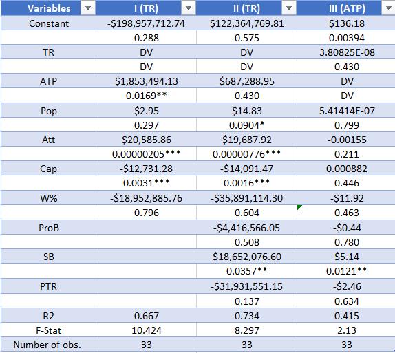
206
that one unit change in Regional Population leads to a $14.83 increase in a Teams Total Revenue. It has not been tested but is assumed that Regional Population and Average Attendance are also positively correlated. This study on Regional Population (fanbase size) aligns with Salaga and Winfree’s (2013) findings that a larger population size of a fanbase correlates with higher revenues for franchises. However, it was found that the size of the team’s Regional Population has a small positive, but no significant effect on the Average Ticket Prices of their team.
Average Attendance (Att) and Stadium Capacity (Cap) are both statistically significant at the 1% level to a Team’s Total Revenue in both models I and II, as expected, as these variables are viewed to be related. The variables do differ in their findings, however. Average Attendance positively influences a Teams Total Revenue. A one-unit change in the Average Attendance over the course of a regular season increases Teams Total Revenue by $20,585.86 in model I, and by $19,687.92 in model II when the variables of prestige are added to the regression model. This finding goes against the trade-off of attendance and profits as mentioned in Brunkhorst and Fenn’s (2010) study. Although in this study, this finding is not surprising as additional attendance corresponds to more tickets being sold and therefore higher revenues, all else remaining equal. This finding is also not a surprise due to the lack of sufficient data found on the operation costs of an NFL stadium. It is assumed that Average Attendance is not as statistically significant with the addition of stadium cost variables. Also, it is assumed that smaller-market franchises benefit more from additional attendance than more established, larger-market franchises. Average Attendance did not play a role in the Average Price of Tickets for an NFL franchise.
Franchises are restricted to the number of tickets they may sell due to the capacity size of their stadiums. The variable Stadium Capacity (Cap) is statistically significant at the 1% level and harms a franchise’s revenue. This finding does not align with previous research (Salaga and Winfree, 2013; Diehl et al., 2015) which states teams with higher capacity stadiums do experience higher profits, however, this study slightly differs. In theory, and as it is assumed, a franchise with a higher capacity stadium should experience higher profits. Although, this study is testing the effects of additional capacity on a team’s revenue, strictly. Therefore, it is clearer why the model displays a unit increase in Stadium Capacity has a -$12,731.28 effect on Team’s Total
207
Revenue in model I, and a -$14.091.47 effect in model II. To produce more capacity a team must spend a high percentage of their revenue, which is why a negative correlation between Stadium Capacity and Team Total Revenue is not unexpected. Again, Stadium Capacity was not found to correlate with Average Ticket Prices.
The only variable found to correlate both Team Total Revenue and Average Ticket Prices, and the only variable that is statistically significant to ticket prices, was Super Bowl Titles (SB). In models I and II respectfully, the Super Bowl Title variable is statistically significant at the 5% level and displays a positive force on both revenue and ticket prices. This is not at all shocking, as this variable is a proxy for the pinnacle achievement in the NFL and is the ultimate measure of prestige. This finding presents the notion that a past team’s performance does indeed impact the revenue and ticket pricing of an NFL franchise. And it is assumed that the number of Super Bowl Titles marginally increases NFL team revenue and ticket prices. Also, whether it be one or multiple Super Bowl wins, the demand for an NFL team’s tickets does skyrocket with a Super Bowl win. From model II, it is indicated that a Super Bowl win translates to an $18,652,076.60 increase in a Team’s Total Revenue. And from model III, fans should expect an increase in the price of tickets of at least $5.14 on average. This finding does align with other studies (Brunkhorst and Fenn, 2010; Salaga and Winfree, 2013; Diehl et al., 2015) as team performance, revenue, and average ticket prices are all positively correlated. Team owners should take note of this variable, as a Super Bowl win not only places an NFL team on a pedestal for league prestige but can also be used as a financial cushion for future seasons. Furthermore, it is assumed that a Super Bowl title is essentially the only trade-off that a fan would accept for higher ticket prices.
Shockingly, Super Bowl Titles were the only variable of prestige to have a statistically significant effect on either Team’s Total Revenue or Average Ticket Prices. Team Winning Percentage (W%), was the most surprising conclusion as it directly goes against the findings of Brunkhorst and Fenn (2013) who tested that previous season winning percentage does play a small, yet significant role on average ticket prices. This study’s result of the winning percentage being statistically insignificant is not concerning, however. As it is cited in Brunkhorst and Fenn’s (2013) findings, previous seasons’ winning percentage is quietly significant due to the franchise owner’s lack of knowledge of how the team will be performing on the field in the
208
upcoming season. This is why it is not concerning that the winning percentage has no correlation to Team’s Total Revenue and Average Ticket Price in this study’s models.
The number of Pro Bowlers (ProB), as a proxy for the number of all-stars on the roster, was found to be negatively correlated, yet statistically insignificant to both Total Team Revenue and Average Ticket Price. This is an unusual finding for this study as it goes against the findings cited in Krautmann and Berri’s (2007) study which established that teams with quality rosters, and teams that play quality rosters more frequently, tend to have higher Average Ticket Prices. Through this study, it is now assumed that teams with higher-quality rosters may have increased ticket prices, although, these teams suffer greater hits to their revenue because of the costs associated with retaining these high-quality players. The findings in this study again align with Brunkhorst and Fenn (2010) as they also found that star players do not play a significant role in a franchise’s total revenue or average ticket price.
As for Pro Teams Within Region (PTR) and the dummy variable for specific divisions, there should be more research and focus done on these topics to ensure that there is no relationship between these variables and Total Team Revenue and Average Ticket Prices. For Pro Teams Within Region, however, could be slightly statistically significant as it is somewhat negatively correlated with Total Team Revenue. More research needs to be done, as there is a possibility that the number of pro teams within an NFL franchise’s region may hinder the demand for NFL game tickets. This is especially a possibility due to the NHL and NBA seasons overlapping with the NFL, and it is assumed that teams from other leagues act as substitutes rather than complements. The dummy variable for specific divisions was omitted from the study as there were no correlations found between specific divisions and Total Team Revenue or Average Ticket Prices.
Unfortunately for this study, there was a lack of sufficient data on other aspects that affect a franchise’s profitability, hence the reason why this study focuses the attention on purely revenue rather than profit. Unlike Krautmann and Berri’s (2007) study, this study was unable to attain sufficient data pertaining to the costs and corresponding revenues of other franchise aspects such as concessions, merchandising, parking, personnel salaries, and marketing. Although, from this limitation, franchise owners can gather a clearer message. For owners, their number one priority should be acquiring the top talent within their team’s financial means, and
209
ultimately, reaching the pinnacle of the NFL by winning a Super Bowl title. From the study, owners may gather and assume that fans’ willingness to pay for tickets, concessions, parking, and merchandising drastically increases when a franchise reaches its ultimate goal of winning the Super Bowl.
6.0 Conclusion
Overall, this study has attempted to gain insights into the determinants of NFL ticket prices as well as the factors that play into an NFL team’s revenue. From this study, it has been found that Regional Population (fanbase size), Average Attendance, Stadium Capacity, and the number of Super Bowl titles all play a factor in an NFL franchise’s revenue. Also, we can conclude that many outside factors that could play a role in a franchise’s revenue often do not also play a role in the determinants of ticket prices. The main factor found in this study to correlate both an NFL franchise’s revenue and ticket prices is Super Bowl titles. It is now undoubtedly a fact that winning a Super Bowl does not only put a franchise on a pedestal in terms of NFL prestige, but it also places a franchise on a financial cushion as well. For NFL owners, their number one priority should be the talent that they are responsible for signing to play on the field, as it is the only factor tested in this study affecting revenue that owners essentially have control over. Moreover, a Super Bowl win is the only trade-off a fan would accept for more expensive tickets. More research on this topic is recommended as there are factors in this study that need more examination. For example, it is assumed that the number of professional teams within an NFL team’s region is detrimental to a franchise’s revenue, as teams from other leagues could be considered substitutes. However, in this study, there were no correlations found between the number of professional teams within the region and team total revenue or average ticket prices.
210
Appendix A: Variable Description and Data Source
Acronym
Description
ATP Average Ticket Price
Data Source
Statista.com
TR Total Team Revenue (2022) Forbes
Pop Regional population for a specific NFL team
Att Average home stadium attendance (2022)
Cap Home field stadium capacity
PTR The number of professional teams in the same region as a particular NFL team
W% Teams 2021 winning percentage
ProB Number of Pro Bowlers (all-stars) on the team roster at the beginning of the 2022 season
SB The number of Super Bowl titles that a franchise has won in their team history
Census.gov
ESPN.com
ESPN.com
Statista.com
ESPN.com
ESPN.com
Statista.com
7.0 Bibliography
211
2020 Census, Demographic Analysis (DA) and Population Estimates for ...
https://www.census.gov/content/dam/Census/library/visualizations/2021/comm/2020census-demographic-analysis-and-population-estimate.pdf.
“Average Attendance of NFL Teams.” ESPN, ESPN Internet Ventures, 2022, http://www.espn.com/nfl/attendance.
Brinsford, James. “The Most and Least Expensive NFL Teams to Follow This Year Revealed.” Newsweek, Newsweek, 8 Nov. 2022, https://www.newsweek.com/nfl-most-leastexpensive-teams-this-year-1757585.
Brunkhorst, John P., and Aju J. Fenn. “Profit Maximization in the National Football League.” Journal of Applied Business Research (JABR), vol. 26, no. 1, 2010, https://doi.org/10.19030/jabr.v26i1.276.
Coates, Dennis, and Brad Humphreys. International Journal of Sports Finance, Morgantown ,se WV, 2007, pp. 161–170, Ticket Prices, Concessions and Attendance at Professional Sporting Events.
Diehl, Mark A., et al. “Price Elasticity of Demand in the Secondary Market.” Journal of Sports Economics, vol. 16, no. 6, 2015, pp. 557–575., https://doi.org/10.1177/1527002515580927.
Gough, Christina. “Most Super Bowl Wins by NFL Team.” Statista, 13 Feb. 2023, https://www.statista.com/statistics/266516/number-of-super-bowl-wins-by-nflteam/?locale=en.
Gough, Christina. “NFL Average Ticket Price by Team 2021.” Statista, 27 July 2022, https://www.statista.com/statistics/193595/average-ticket-price-in-the-nfl-by-team/n.
Gough, Christina. “NFL Revenue by Team 2021.” Statista, 2 Jan. 2023, https://www.statista.com/statistics/193553/revenue-of-national-football-league-teams-in2010/.
Krautmann , Anthony, and David Berri. “Can We Find It At The Concessions? Understanding Price Elasticity in Professional Sports.” Sagepub, Journal of Sports Economics , 2007, file:///C:/Users/student/Downloads/Can_We_Find_It_at_the_Concessions_Understanding_ Pr.pdf.
Kuznitz, A.J. 2011, Professional Sports Teams and Their Local Economic Impact, https://digitalcommons.coastal.edu/cgi/viewcontent.cgi?article=1103&context=honorstheses. Accessed 10 Apr. 2023.
“National Football League Standings.” NFL.com, https://www.nfl.com/standings/league/2022/reg.
212
“NFL Pro Bowlers by Team .” NFL Communications, https://nflcommunications.com/Pages/Rosters-Announced-For-2022-Pro-Bowl-PresentedBy-
Verizon.aspx#:~:text=Five%20teams%20%E2%80%93%20the%20BALTIMORE%20RA VENS,on%20the%20Pro%20Bowl%20roster.
“North American Sport Franchises.” A List Showing Which Cities Have Major League Sports Franchises, 2022, https://www.stadium-maps.com/facts/sports-franchises.html.
Salaga, Steven, and Jason A. Winfree. “Determinants of Secondary Market Sales Prices for National Football League Personal Seat Licenses and Season Ticket Rights.” Journal of Sports Economics, vol. 16, no. 3, 2013, pp. 227–253., https://doi.org/10.1177/1527002513477662
“Sports Money: 2022 NFL Valuations.” Forbes, Forbes Magazine, https://www.forbes.com/nflvaluations/list/#tab:overall.
213
An Empirical Analysis of the Effects of Government
Influence on Deforestation in Latin America
Francine Roberge
Abstract:
This paper investigates government influence and factors that may increase the rate of deforestation in Latin American countries. An empirical analysis will be conducted to measure the change in deforestation rates based on several potential influences. The analysis will look specifically at countries in Latin America that have a high level of deforestation including Argentina, Bolivia, Brazil, Columbia, Paraguay, Peru, and Venezuela from 1996 until 2011. Variables studied include accessibility, suitability for agriculture production, corruption perception, government effectiveness, political stability, GDP per capita, foreign direct investment, and trade openness. The results show that as more forest cover is lost, and higher rates of deforestation occur, the government institution becomes more corrupt and less politically stable. Additionally, when there is less foreign direct investment, there is also lower rates of deforestation due to the recently diminished levels of natural resources in the area.
JEL Classification: Q23, O13, H10, F10, D73
Keywords: Deforestation, Economic Development, Structure and Scope of Government, Trade, Corruption
a Department of Economics, Bryant University, 1150 Douglas Pike, Smithfield, RI02917.
Email: froberge@bryant.edu
214
1.0 INTRODUCTION
Climate change continues to become a more urgent matter for policymakers as well as leaders alike. Particularly in Latin America, climate issues are of great importance. Most agricultural production in this area relies on their vast rainforests. However, this region is seeing a rapid decrease in the amount of forest area, at a great rate than the rest of the world. This may be due to many factors, but one specific reason that can explain for this inconsistency is corruption amongst leaders within these countries. Bringing attention to this matter may help slow the destruction of the rainforests in these regions.
This study aims to enhance understanding of the high rate of deforestation in Latin American countries and the role that government influence plays on it. From a policy perspective, this analysis is important because if there is a strong direct relationship, by reforming government and corruption, then the rainforests can be saved, and therefore the effects of climate change can be slowed or even reversed in the coming years. The relevance of this study is that climate change is becoming an increasingly pressing problem with no immediate and easy solution. Therefore, any insight into this issue can help aid policymakers in future decisions and help stop the slow now.
As deforestation becomes a more pressing problem, not only is biodiversity decreasing and the environmental health taking a toll, but the citizens of these countries are also negatively affected. In both Latin America and the Caribbean, the increase in deforestation is leading to higher rates of outside agriculture and can in turn put those who depend on the forest land of their livelihood in a tough state. Not only do they no longer have access to resources they used to, but now there is more industry in their space leading to a potential increase in poverty and hardship for these individuals. Some specific areas can be investigated to help address the issues posed by deforestation of the rainforests are the strength of government in the country, amount of FDI, trade openness within the borders, and the amount of corruption that occurs. Various studies and papers have addressed this problem and have looked into the causes of the increased rate of deforestation.
This paper will look at Latin American countries from the years of 1996 to 2011. In this time period, Latin America faced a disproportionate amount of deforestation compared to other
215
regions in the world. Factors that may be escalating the amount of deforestation in these areas include the strength of the institutions and their ability to lead and govern a country. The stability as well as the intentions of those in power can greatly impact what foreign influences can enter the country as well as what is done with the country’s natural resources.
2.0 FOREST COVER AND FDI TRENDS
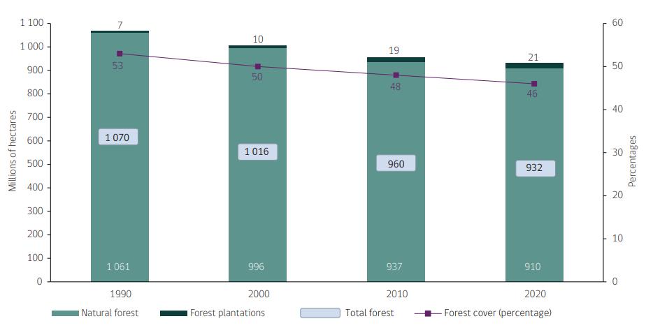
United Nations ECLAC
Figure 1 shows the amount of forest cover in Latin America and the Caribbean. The figure shows the years 1990-2020 and displays both the actual coverage in millions of hectares as well as the percentage of cover for this region. It also depicts how much of the coverage is natural forest and forest plantations. Natural forests are forests that are naturally occurring, whereas forest plantations are forests that are planted usually of a singular tree variety for the purposes of timber and other sources of production. The diagram shows that since 1990, the forest cover percentage has been decreasing steadily at around 2-3% every 5 years. Since 1990, the total percentage of forest cover has decreased by 7%. Similarly, the amount of natural forest has also decreased whereas the among of forest plantations has increased. Although that indicates an increase in trees, these trees are being planted with the intent of cutting them down, so they are not addressing the problem at hand.
Figure 1: Forest Cover in Latin American and the Caribbean
Source:
216
Figure 2: Global FDI Flows in Latin America and the Caribbean
Source: ECLAC and UNCTAD
Figure 2 shows the Global FDI flows for Latin America and the Caribbean from the years 1990 to 2017. It shows the flows in both billions of dollars on the left, and the percentage of investment on the right. In addition, it breaks down the amount of investment for each type of economy: transition, developed, and developing. Since 1990, the amount of FDI for all types of economies has increased. In 2001, there was a large dip in the amount of FDI for developed countries due to the global slow of economic growth (UNCTAD, 2002). Another notable trend is the emergence of transition economies and investment in them. Starting in 2002, a level of investment occurs in this type of economy, indicating expansion, growth, and positive expectations by foreign investors. Although foreign direct investment is still occurring, it is not increasing at the same rate that it has been in years prior.
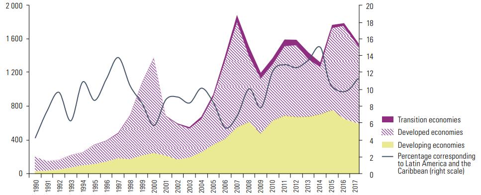
3.0 LITERATURE REVIEW
Deforestation is continuing to become a larger problem across the globe Hit particularly hard by this epidemic is Latin America and the Caribbean In this area, there is a high density of trees and rainforests. In addition, the industry and economies in these countries depend heavily on the rainforests for production and an inflow of funds. Deforestation is bad for the environment and disrupts the natural ecosystems that exist there, but it also leads to an increase in global warming effects which is becoming an increasingly larger problem within the world. The damaging of forests disrupts soil stabilization, water conservation, and may lead to more
217
desertification (Assa, 2020). This can also interrupt already in place agricultural processes which are necessary to sustain life as well as for economic stabilization. Although deforestation is the issue at hand, there are many factors that can be studied to see the effects that they have on the issue. For example, the strength of government in the country, amount of FDI, trade openness within the borders, and the amount of corruption that occurs. Various studies and papers have addressed this problem and looked into the causes of the increased rate in deforestation.
First, foreign direct investment plays a large role in the amount of deforestation that occurs in a country. Foreign direct investment, or FDI, is the amount of funding that comes from investors outside of the home country. They provide funds from a foreign country into a business venture within the home country. With this investment, they in turn get control of the good or resource within the country. Over the past 25 years, the amount of foreign direct investment in Latin America and the Caribbean has been increasing steadily (ECLAC, 2018). With this inflow of money into the economy, outside factors now have a say in resources like rainforests. More of this land is being converted into forest plantations as well as just being destroyed for the purposes of increasing the amount of agricultural land (ECLAC, 2021). These are more of cash cow ventures than the natural forests are, and therefore are more attractive than the natural forests that stand there. Therefore, foreign direct investment is having a negative effect on the forests. A variable that ties into this is trade openness as well. Being tied into trade arrangements like NAFTA (North American Free Trade Agreement) and other more localized trade agreements, it makes FDI in these countries that much more attractive for it is easier to get resources across borders and increase the flow of funds (Congressional Research Service, 2020).
Another variable that is playing a large role in deforestation is the role political institutions play in each respective country. Whether there is a strong government or not makes a big difference. Within Latin American countries there has been high rates of corruption, low rates of political stability, and low to moderate rates of government effectiveness rates. Looking at these variables can help form a good view into how each country’s economy operates and where their priorities lay. In corrupt government situations, money and power rule. When this occurs, it is much more likely that environmental endeavors take a back seat, and this is becoming apparent as the rate of deforestation in these regions continues to increase at an
218
alarming rate (Moreira-Dantas and Soder, 2021). With the decrease of trees and the increase of agricultural practices and other increasing industries, the climate becomes more polluted due to the rising rates of damaging carbon dioxide emissions according to Galinato and Galinato in 2011. Although this may be a global concern, when there is weak political control, it is difficult to create any legislation or change the way that these natural resources can be protected and therefore benefit the environment and world as a whole.
4.0 DATA AND EMPIRICAL METHODOLOGY
4.1 Data
The study uses panel data from 1995 to 2011. Data were obtained from the World Development Indicators from the World Bank.
1 Summary Statistics
Variable Observation Mean Std. Dev. Min Max LOGCHANGE 112 -0.00623 .00447 -0.02186 -0.00152 CPI 112 -0.54433 .40584 -1.4454 .1457 STABLE 112 -0.77669 .59392 -2.39011 .286 GOVEFF 112 -0.43704 .38725 -1.145 .329 LOGSUIT 112 13.0162 .92103 11.8962 14.65947 LOGGDP 112 8.13319 .697076 6.7892 9.524633 LOGFDI 112 1.269 .5792 -1.387 2.5799 LOGTRADE 112 3.7349 .41947 2.7481 4.4516 219
Table
4.2 Empirical Model
Following Moreira-Dantas and Soder (2022) this study adapted and modified their empirical model. Influences from Galinato and Galinato (2011) like corruption control and political stability, were added to this model as well The model could be written as follow, where t represents time, and i indexes countries:
LnChangeForestAreai,t
The dependent variable of the model is natural log change in forest area. Log Change in Forest Areai,t, from country i at year t, measures the change in forest area cover from year to year. Starting in 1995 until 2011, the change in forest cover is reported for each of the 7 countries in Latin America. The log was taken of this variable so that the data better fit the model. A negative value for all data points, shows that regardless of the country, over time, the amount of forest cover is decreasing.
Independent variables consist of seven variables obtained from the World Bank. Appendix A and B provide data source, acronyms, descriptions, expected signs, and justifications for using the variables. First, CPI (size of country at year ) represents the Corruption Perception Index. This variable asks citizens how corrupt they view their own country’s government system. STABILITY represents Political Stability. This also asks citizens how politically stable their country’s government seems. GOVEFFECT represents government effectiveness, and how effective the home government seems in creating policy and functioning as a whole as viewed by their citizens. LOGSUITABILITY, takes the natural log of Agriculture Land Suitability. This variable measures the land’s ability to reach potential yields in a variety of different crops. LOGGDP, takes the natural log of GDP per Capita in USD. This is measured by taking the GDP and dividing it by the total number of citizens in each respective country. LOGFDI takes the natural log of Foreign Direct Investment. This is the total level of direct investment from foreign entities in each country. The last independent variable is LOGTRADE.
= β0 + β1CPIi,t+ β2Stabilityi,t+ β3GovEffecti,t+ β4LnSuitabilityi,t+ β5LnGDPi,t+ β6LnFDIi,t+ β7LnTradei,t+ ε
220
This is measured by taking the natural log of Trade Openness. Trade Openness is measured by taking a country’s total exports and imports and dividing the total by the country’s GDP.
5.0 EMPIRICAL RESULTS
Table 2: Regression results for Latin American Countries
Note: *** , **, and * denotes significance at the 1%, 5%, and 10% respectively. Standard errors in parentheses
Log of Forest Change I (FE) II (RE) CONSTANT .391*** (.086) 0.43*** (0.121) CPI -.00125 (.0008) -.00313** (.0013) STABILITY - 00047 (.0007) -.00152** (.00067) GOVEFFECT -.00185* (.001) -.0001 (.0016) LNSUITABI LITY -.0305*** (.0066) -.00273*** (.0006) LNGDP -.00059* (.00033) .00022 (.00052) LNFDI 0 00047 (.00032) .0024*** (.000648) LNTRADE -0.002** (.0007) -.00483*** (.00133) R2 0.0311 0.7162 F-statistic/Chi 6.02*** 116.71*** Number of obs. 112 112
221
The empirical estimation results are presented in Table 2. The empirical estimation shows both the fixed effects and random effects of the regression. The fixed effects regression has a very low R2, 0.0311, indicating that the model does not account for a lot of the variations in data. The random effects regression has a much higher R2, 0.7162, indicating that the model accounts for a much higher percentage of the data The random effects model measures the effect of time over the regression. In this case, the random effects regression indicates that over time the relationship between the dependent and independent variables is changing and is significant. Random effects assumes that unobserved variables are uncorrelated with the model. This can be problematic and lead to potential biases.
Looking specifically at the random effects model, there were 5 significant variables in addition to the constant variable also being significant. This implies that this model produces results that are meaningful and can be interpreted and applied to prior research. Some of the independent variables do have a relationship that can be interpreted and have significance when compared to the dependent variable, log of area of forest change.
First, CPI, or the corruption perception index, is significant at the 5% level. It has a coefficient of -0.00313. This implies that for every 1% change in log of forest area, there is a 0.00313 decrease in CPI. Therefore, as the amount of forest area decreases, the more corrupt an institution is perceived to be by its citizens. Similarly, Stability is also significant at the 5% level and has a coefficient of -0.00152. This implies that for every 1% change in log of forest area, there is a 0.00152 decrease in Stability. As forest cover decreases, the government is perceived as being less stable by its citizens.
Next, the log suitability variable is significant at the 1% level and has a coefficient of.00273. This implies that for every 1% change in the forest area, the land suitability amount decreases by 0.00273%. Therefore, as there is less forest area, the land becomes more suitable for agricultural processes. This may be because now that forests are cleared so there are more fields available for farming, increasing the suitability level of the land.
Log FDI is another significant variable at the 1% level It has a coefficient of 0.0024. This implies that as Log change in forest area changes by 1%, the log of FDI will increase by 0.0024%. The two variables have a positive relationship showing that as the amount of forest
222
area increases, so does the amount of FDI. This is consistent with research (ECLAC, 2018). FDI inflows have been gradually declining from their 2011 peak. 90% of this decline has occurred in the natural resources sector (ECLAC, 2018). Therefore, this finding is consistent with the regression because as the amount of forest area decreases, so does the number of natural resources. Therefore, FDI should also be diminishing
The last significant variable in the random effects model is the log of openness to trade. This is statistically significant at the 1% level and has a coefficient of -0.00483. This implies that as forest area cover changes by 1%, the openness of a country to trade decreases by -0.00483%. Therefore, as there are less trees, countries are more willing to trade. This can be due to a better running economy due to more opportunities and places to expand production with the less forested areas.
Interpreting these results from the relative changes of the independent variables, it is clear that the weaker the government institution is in a country, the more susceptible the area is to outside factors and therefore the amount of forest area is at risk. With outside interest looking to capitalize from the land, they are more likely to come in and use the land for its resources and make money, rather than looking to preserve the nature that is already there. Likewise, weaker institutions that are potentially more corrupt, are more likely to allow this business ventures to enter and use the land for they are potentially receiving kickbacks from the ventures. They may not have the people’s best interest in mind, but rather are looking out for what will further their desires.
Limitations of the study include sample size and data available. There was limited data available making it difficult to extrapolate results. In addition, the variables CPI, Stability, and Government Effectiveness, are all based on a subjective scale. They are measured using current citizens’ perceptions. It is uncertain how large the sample size is and whether or not it is comprehensive of the whole population. Likewise, if it is a more unstable and corrupt area, citizens may not want to share their true feelings due to the possibility of their being dangerous consequences. Specifically looking at the model, there may be omitted variables making it difficult to tell how accurate it is and whether or not the findings can be expanded to other countries and regions.
223
The study also has policy implications that can be addressed. There is an overall trend of decreased forest area over time regardless of country and the government system that they have. Global warming is becoming a more urgent matter and the amount of decreasing forest cover is only adding to the issue. Looking at the model, areas with a higher level of corruption, more suitable land, and more FDI tend to lose land at a quicker rate compared to areas that have less agriculturally productive land, and therefore less foreign interest. This finding has policy implications for a stronger government presence can help slow or stop the growing rate of deforestation. Areas with nutrient-rich land need to be protected for there is more interest in using and developing them. Therefore, stronger government programs or more environmentally focused programs can help form legislation that can protect this land from being developed, and let it continue to be natural and help the environment sustain itself.
6.0 CONCLUSION
In summary, over time the amount of forest cover is decreasing in Latin American countries. There are ties between the rate of deforestation being higher when there are more corrupt institutions in control. This can be looked at for policy implications and the future of forests. Climate change is becoming an increasing problem across the world and one step that can be taken to slow the issue is controlling institutions and looking at the role that they are playing.
Overall, those that care purely about economic expansion may be targeting areas like Latin America for their robust natural resources and potential ease of entry due to their weak institutions. However, identifying the reasons behind increased deforestation can hopefully curb the rate at which it is occurring. From this model, the argument for the need of stronger institutions can be made. In order to save the rainforests, slow the rate of global warming, and stop more harmful emissions from entering the atmosphere, there needs to be more regulations and a stronger presence of the government within industrial practices. In addition, having stricter practices and screening of potential investors before allowing business within the country could help slow this process and understand what they are necessarily interested in.
224
Although the growing of the economy in developing countries is very important, in this instance growing them for the sake of growing them may not be the answer. Destroying natural resources and polluting the environment may not be the best course of action. It may help in the short run, but in the long run depleted natural resources and a strong dependence on foreign investment may ultimately hurt these countries.
225
Appendix A: Variable Description and Data Source
Acronym Description
LNFORESTAREA By how much the forest area changed in a year, calculated by taking the percentage change.
CPI Rated on a scale of -2.5-2.5, how corrupt gov’t seems to citizens.
STABILITY Rated on a scale of -2.5-2.5, how stable the gov’t seems to citizens.
GOVEFFECT Rated on a scale of -2.5-2.5, how effective gov’t seems to citizens.
LNSUITABILITY Land’s ability to reach potential yields in a variety of crops.
LNGDP The GDP divided by number of citizens, measured in USD.
LNFDI Total amount of direct investment from foreign entities into the home country’s economy.
LNTRADE Measure of exports and imports divided by the country’s GDP.
Data source
World Bank
World Bank
World Bank
World Bank
World Bank
World Bank
World Bank
World Bank
226
Appendix B: Variables and Expected Signs Acronym
LNCHANGE
By how much the forest area changed in a year, calculated by taking the percentage change
CPI Rated on a scale of2.5-2.5, how corrupt gov’t seems to citizens.
STABILITY Rated on a scale of2.5-2.5, how stable the gov’t seems to citizens.
GOVEFFECT Rated on a scale of2.5-2.5, how effective gov’t seems to citizens
LNSUITABILITY Land’s ability to reach potential yields in a variety of crops.
LNGDP The GDP divided by number of citizens, measured in USD.
LNGFDI
Total amount of direct investment from foreign entities into the home country’s economy.
LNTRADE Measure of exports and imports divided by the country’s GDP.
Decrease in size of forests -
Corruption in Governments -
Stability in Governments -
Effectiveness of Governments -
How suitable the land is for agricultural production
+
GDP per capita +/-
The amount of FDI that a country is receiving. Helps gauge other countries and investor’s interest
+/-
A country’s openness to trade with other nations -
Variable
Expected
Description What it captures
sign
227
BIBLIOGRAPHY
Assa, B. (2020). The deforestation-income relationship: evidence of deforestation convergence across developing countries. Environmental and Development Economics, 26, 131150. doi:10.1017/S1355770X2000039X.
CRS. (2020). The Committee on Foreign Investment in the United States. CRS Report, RL33388. https://crsreports.congress.gov/product/pdf/RL/RL33388.
ECLAC. (2018). Foreign Direct Investment in Latin America and the Caribbean moves away from natural resources. ECLAC keynotes for development, No.3.
https://repositorio.cepal.org/bitstream/handle/11362/43423/1/S1800258_en.pdf
ECLAC. (2021). Forest loss in Latin America and the Caribbean from 1990 to 2020: the statistical evidence. ECLAC Statistical Briefings, No.2.
https://repositorio.cepal.org/bitstream/handle/11362/47152/1/S2100265_en.pdf.
Galinato, G. & Galinato, S. (2011). The effects of corruption control, political stability and economic growth on deforestation-induced carbon dioxide emissions. Environmental and Development Economics, 17, 67-90. doi:10.1017/S1355770X11000222.
Moreira-Dantas, I. & Soder, M. (2022). Global Deforestation Revisited: Role of weak Institutions. Elsevier, 122. https://doi.org/10.1016/j.landusepol.2022.106383
UNCTAD. (2002). FDI DOWNTURN IN 2001 TOUCHES ALMOST ALL REGIONS. UNCAD Press Release, 36. https://unctad.org/press-material/fdi-downturn-2001-touches-almost-allregions.
Walker, R. (2004). Theorizing Land-Cover and Land-Use Change: The Case of Tropical Deforestation. International Regional Science Review, 27(3), 247-270. DOI: 10.1177/0160017604266026.
228
An Empirical
Analysis of Prime Performing Age of NBA Players; When Do They Reach Their Prime?
Tony Salameh
Abstract:
This empirical research paper investigates the prime performing age of NBA players from the perspective of General Managers. The study aims to identify the age range in which players are most effective on the court and to determine if there is a significant relationship between age and player performance. Player performance statistics data was collected from ESPN and analyzed to help determine at what age players reach their prime productivity levels for a team. The findings suggest that the prime performing age of NBA players is between 27 and 31 years old, with a slight decline in performance after the age of 32. The results have important implications for team management and player recruitment strategies.
JEL Classification: Z2
Keywords: Prime Performing Age, NBA, Star Players
a Department of Economics, Bryant University, 1150 Douglas Pike, Smithfield, RI02917. Phone: (508) 494-8459. Email: asalameh@bryant.edu.
229
The NBA is one of the most popular professional sports leagues in the world, with millions of fans following their favorite teams and players each year. One of the most important factors that determine the success of an NBA team is the performance of its players, and the age of the player is a crucial factor in this regard. Over the years, NBA teams and General Managers have used various strategies to acquire and retain players in their prime, with the aim of building a successful and competitive team. This empirical analysis aims to examine the effects of prime performing age of NBA players and how this affects their value in the eyes of the General Managers' player acquisition and team building strategies.
The prime performing age of an NBA player is a topic of much debate and speculation among fans, players, coaches, and General Managers. Some argue that players peak in their early 20s, while others believe that players can continue to perform at a high level well into their 30s. However, determining the prime performing age of an NBA player requires empirical analysis that considers various factors such as player statistics, team performance, and injury history. The results of such analysis can provide valuable insights to General Managers when making decisions about player acquisitions and team building strategies.
General Managers play a critical role in the success of an NBA team, as they are responsible for identifying and acquiring players that fit into the team's overall strategy and goals. This requires an understanding of the prime performing age of NBA players and how it affects their performance on the court. By analyzing the effects of prime performing age on NBA players, General Managers can make informed decisions about player acquisitions and roster management, which can ultimately lead to a more successful and competitive team. Overall, this empirical analysis aims to provide a comprehensive understanding of the prime performing age of NBA players and its effects on General Managers' player acquisition and team building strategies.
By using statistical models to analyze player performance data from the 20002010 seasons, this study can provide valuable insights into how a players age can influence player overall value and help General Managers make more informed decisions about player acquisitions and roster management. Ultimately, this research can contribute
1.0 INTRODUCTION
230
to the ongoing debate surrounding the prime performing age of NBA players and provide valuable information to NBA teams and General Managers as they strive to build successful and competitive teams.
This paper is guided by the ongoing studies to that investigate player value based on performance age and other factors such as movement in the market. Specifically aiming to correlate players age to their performance and when they hit their “prime age.”
The rest of the paper is organized as follows: Section 2 gives a brief literature review. Section 3 outlines the empirical model. Data and estimation methodology are discussed in section 4. Finally, section 5 presents and discusses the empirical results. This is followed by a conclusion in section 6.
2.0 Evolution of Player Age
Figure 1 shows a graph of the NBA All-Star selected players and their age for the past 70 years. We see that the most talented players are usually in the age range of 26-29, however there are years in which the average age has risen and fallen tremendously. This range remains quite similar to the expected ranges from the articles above.
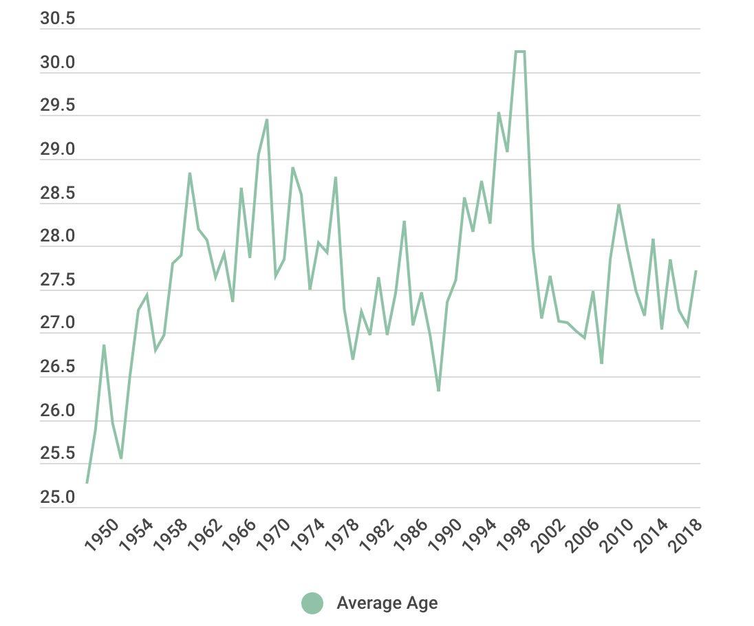 Figure 1: All-Star Players Average Age
231
Source: Hoop Hall Data Base
In the NBA, there have been several trends over the years regarding the prime performing age of players. Traditionally, players were thought to reach their peak performance in their late 20s or early 30s, but recent trends suggest that players are hitting their prime at a younger age. This is believed to be due to increased training at a young age and better player development.
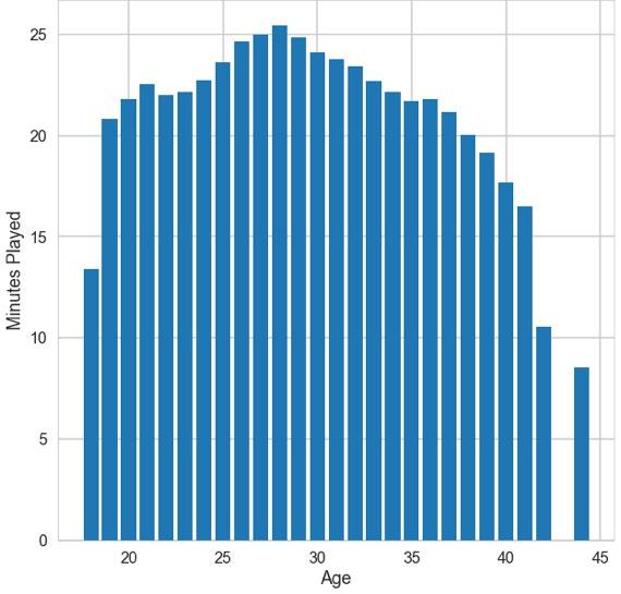
One trend that has contributed to this shift is the increased focus on player development and training from a young age. Many NBA players now enter the league after playing in high-level AAU and college programs, where they receive top-notch coaching and access to advanced training facilities. In Figure 2 we see that more minutes are being played by younger athletes with the most minutes being played by players age 29.
Another theory that has contributed to younger players reaching their prime is the evolution of the game itself. The NBA has become more focused on athleticism, speed, and skill, and players who possess these qualities are now more highly valued than ever
Figure 2: Minutes Played by Age (2006-2017)
Source: Harvard Sports Analysis Collective
232
before. This has led to teams placing greater emphasis on acquiring and developing younger players who have the potential to become elite athletes.
In recent years, the NBA has also seen a rise in the use of advanced analytics and data-driven decision making. Teams are using sophisticated algorithms and statistical models to evaluate player performance, which has led to a greater emphasis on finding and developing players who have the potential to become elite athletes at a young age. Overall, the trends in the NBA suggest that players are reaching their prime at a younger age, and that teams are placing greater emphasis on player development and data-driven decision making in order to find and develop the next generation of elite athletes. As the game continues to evolve and change, it will be interesting to see how these trends continue to shape the NBA and the way we think about player development and performance.
3.0 LITERATURE REVIEW
The National Basketball Association (NBA) is a highly popular and profitable professional sports league worldwide, with teams and players attracting significant attention and financial rewards. Among various factors that determine player salaries, player age plays a crucial role, with teams and players placing great emphasis on the concept of the "prime age" in the NBA. This literature review will explore several articles that examine the relationship between age and performance, with a particular focus on the prime age period, and its implications for player development and team success.
Arkes and Karolak (2019) conducted an analysis of NBA salaries and player age using data from the 2016-2017 season. They found that player age had a statistically significant negative effect on salary, with older players earning lower salaries than younger players. Additionally, the authors found that the relationship between age and salary varied by position, with point guards experiencing the smallest decline in salary as they aged, and centers experiencing the largest decline. Similarly, Schmidt and Berri (2018) studied the relationship between age and productivity in the NBA using data from the 2013-2014 season. They found that while older players do tend to experience declines in productivity, the effect is relatively small, and many players continue to perform at a high level well into their 30s. The authors
233
suggest that teams may be too quick to let go of older players, and there may be a market inefficiency that could be exploited by teams willing to invest in older players.
Lavoie and Ehrmann (2016) used a nonparametric statistical approach to examine the relationship between player age and productivity in the NBA. They found that older players tend to experience declines in productivity, but the decline is not as steep as previously thought. The authors suggest that teams may be underestimating the value of older players and may be too quick to replace them with younger players.
Taken together, these articles suggest that age is an important factor in determining NBA player salaries, but the relationship between age and productivity is complex. The prime age period represents the period when players are generally believed to be in their physical prime and able to perform at their highest level. As the Arkes and Karolak (2019) study showed, teams may be willing to pay a premium for players in this age range, while players may be more likely to negotiate for higher salaries during this period.
The findings of Lee et al. (2017) have implications beyond salary determination, as they highlight the importance of the "prime age" window for athlete success. Understanding the factors that contribute to athlete success during this period could inform player development strategies, team recruitment and retention practices, and other related issues. Therefore, the intersection of age and performance in sports economics is an important area of research with significant implications for both athletes and sports organizations. Teams and players need to be thoughtful and strategic in their approach to age and performance, considering individual factors such as position, playing style, and injury history to maximize the benefits of the prime age period for player development and team success.
4.0 DATA AND EMPIRICAL METHODOLOGY
4.1 Data
The study uses data from the 2000 to 2010 NBA seasons that has been collected from ESPN and Basketball-Reference.com which are two sports databases where players in-game statistics can be found. Summary statistics for the data are provided in Table 1.
234
From authors Calculations
4.2 Empirical Model
The Empirical Model used in this study follows models creates by Lee et al. (2017) and Schmidt and Berri (2018) and highlights the relationship between Performance and Age as follows:
To analyze the prime performing age of NBA players over the last 10 seasons, the following empirical model can be used:
PER is the Player Effecicey Rating which is a method of determining a player's impact on the game by measuring their per-minute performance. The formula for PER considers the player's positive contributions, such as points, assists, rebounds, steals, and blocks, as well as their negative contributions, such as turnovers, missed shots, and fouls. The formula is quite complex and involves many different variables, including made three-pointers, made field goals, made free throws, offensive and defensive rebounding percentages, steals, blocks, and personal fouls. It also factors in the value of each possession and adjusts for the number of assists based on the team's shooting percentage. To calculate PER, you need to use the complete formula, but the idea is that a higher PER indicates a more efficient and effective player. PER can be used to compare the performances of different players within a team or across the league. It is a useful tool for coaches, scouts, and fans to evaluate player performance and make decisions about
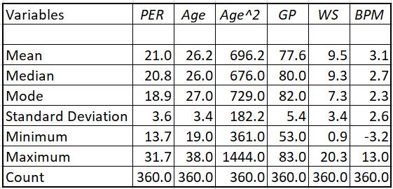
Table 1 Summary Statistics
PER=
+
β0 + β1AGE+ β2AGE^2 + β3GP + β4WS
β5BPM + ε
235
strategy, playing time, and roster moves. However, we were able to gather the calculated PER from the databases. Using the PER as the dependent variable derived directly from the work done by Lee et al. in their study in 2017 to help get a better understanding of player efficiency similar to this study.
Independent variables consist of five variables obtained from basketballreference.com “NBA Statistics” dataset. Appendix A provides acronyms, descriptions, and justifications for using the variables. First, Age represents the age of the player in the current season that the data is being collected in. Next, Age^2 (age squared) represents the player development, knowledge, and skillset that must be accounted for as players mature in the league and have a better understanding of the game. GP represents the number of games played by each player each season. Fourth, WS represents the win share which is a statistic used in the NBA to measure a player's overall contribution to their team's wins. It calculates the number of wins that a player contributes to their team above what a replacement-level player would contribute, taking into account a player's offensive and defensive performance that contributed to the team’s performance. Lastly, BPM represents Box Plus Minus which evaluates players' quality and contribution to the team from a play-by-play regression.
5.0 EMPIRICAL RESULTS
The empirical estimation results are presented in Table 2. The empirical estimation shows a positive relationship throughout all the variables that are present in the regression, however only a few are statistically significant. We see that Age, WS (Win Share), and BPM are all statistically significant and influence a player’s overall value to their team.
236
Table 2: PER Regression Results
Note: * denotes variables that are significant at the 1%. Standard errors in parentheses Source: From authors calculation
The findings in this study show similarities to the studies done by Lee et al. (2019) and Lavoie and Ehrmann (2016) finding that PER, AGE, and WS were all significant factors in analyzing prime performance. To further analyze at what age is “Prime” performing age we take the significant variables and look at pivot charts to see what age range we find the most productivity from players.
Variable Result Age .00014* (.001) Age^2 .46013 (.0006) GP .57601 (.0141) WS .00096* (.0673) BPM .00019* (.086)
237
From analyzing the data and regressions we are able to find an age range that we can statistically prove to be the “Prime” age range in the NBA. We see from Figures 3,4,&5 that the most productive ages in the NBA range from 23-27, with a sharp decline at age 29. The findings align with the predictions from Arkes and Karolak (2019) in which they proved that coaches are willing to pay premium for players in this age range since they believed this was the prime age range.
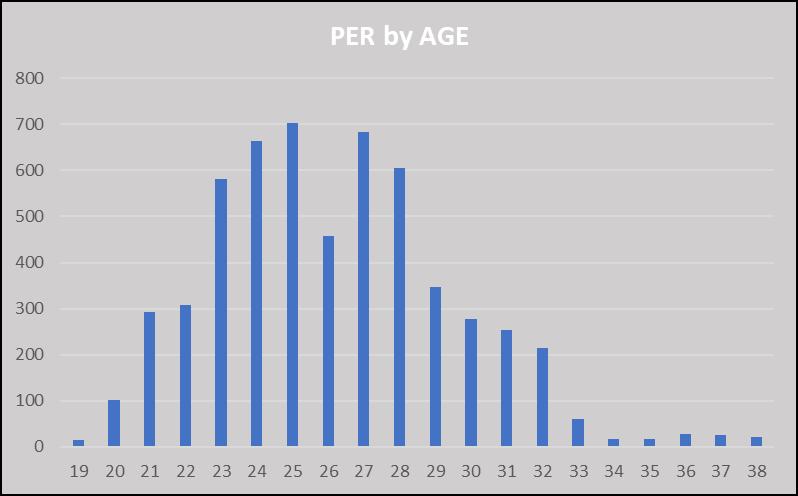
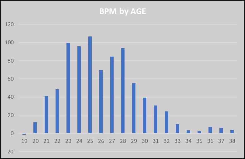
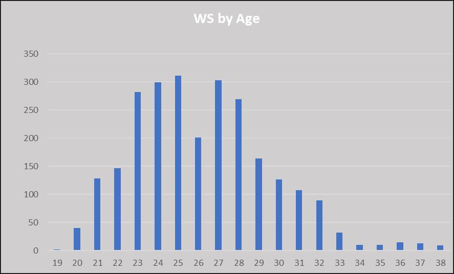 Figure 3: Win Share by Age
Figure 4: Player Effiency Rating by Age
Figure 5: Box Plus Minus by Age
All figures from authors calculation
Figure 3: Win Share by Age
Figure 4: Player Effiency Rating by Age
Figure 5: Box Plus Minus by Age
All figures from authors calculation
238
5.1 LIMITATIONS
The study on the factors of prime performing age in the NBA faces several significant limitations that could affect the validity of its findings. Firstly, the sample size used in the study is relatively small, which may limit the validity of the results.
Secondly, the data used in the study is susceptible to selection bias. For example, we used an initial quantile regression to find the top 30 players from each season to further examine. Moreover, the sample of players used in the study may not be an accurate representation of the entire population of NBA players, which could affect the validity of the results.
Finally, the study lacks control variables that could influence the age at which NBA players perform at their best. While the study analyzed several factors that could affect prime performance age, other variables, such as injuries, team chemistry, and player psychology, could also influence performance but were not included in the analysis. This omission may lead to omitted variable bias, potentially affecting the accuracy of the conclusions drawn.
While the study provides insights into the factors that could affect prime performing age in the NBA, its limitations highlight the need for further research that accounts for a larger sample size, more diverse teams and players, and a wider range of control variables to enhance the generalizability and reliability of the findings.
5.2 Policy Implications
Furthermore, the research indicates that the prime age of talent is getting younger over time, which may have implications for the league's policies. The "one-and-done" rule was implemented to give players more experience before entering the league, but our findings suggest that younger players are prevailing in the league. It will be interesting to see what policies the NBA may put into place next to address this trend and ensure a balance between experience and youth. An idea that may help with player development league wide is waiving this one and done rule so that younger talent (if seen as NBA ready) can enter the league right after completing high school.
239
6.0 CONCLUSION
The purpose of this empirical analysis was to contribute to the ongoing research of data-driven decision making in identifying and developing young talent in the National Basketball Association (NBA). Through an examination of player statistics and various performance indexes over five seasons, we have found that the prime performing age in the NBA ranges between 24-27 years old, with a slight decline in productivity at the age of 29. Our findings confirm the notion that basketball is a sport where players tend to peak in their mid-20s, which has important implications for NBA general managers in terms of talent acquisition and roster construction.
Our study has shown that general managers should take player age into consideration as a bigger factor in their overall value to the team. By altering their approach to talent acquisition based on the prime performing age range, teams can maximize player development and improve their chances of success. Additionally, our analysis suggests that younger players are becoming increasingly valuable in the NBA due to the evolution of the game, which is now valuing athleticism and speed more than ever before.
In conclusion, this study provides valuable insights into the prime performing age in the NBA, which has practical implications for general managers and the league. By using data-driven decision making and considering the prime age range when acquiring talent, teams can optimize their chances of success. Future research should continue to examine the evolving relationship between age and performance in the NBA to ensure that teams remain competitive, and the league continues to evolve.
240
Appendix A: Variable Description and Data Source
Acronym Description
PER Player Efficiency Rating: a method of determining a player's impact on the game by measuring their per-minute performance.
Data source
AGE Player’s age used to interpret age of player each season to help identify prime age
Kaggle Sports Database
ESPN
AGE^2
Age Squared accounts for all other aspects that come with aging such as gained knowledge, skill development and maturation
GP Games Played: Represents the number of games that a player take part in each season
WS Win share: a secondary measure of player value to a team and the success that must be accredited to an individual for each win
BPM Box Plus Minus: evaluates players' quality and contribution to the team from a play-by-play regression
Kaggle Sports Database
Kaggle Sports Database
Kaggle Sports Database
Kaggle Sports Database
Kaggle Sports Database ESPN
241
BIBLIOGRAPHY
Arkes, J., & Karolak, M. (2019). An Analysis of NBA Salaries and Player Age. Journal of Business and Economic Perspectives, 46(1), 47-61. doi: 10.1177/0737469118802669
Brady, B. (2017). WHAT HAPPENS TO NBA PLAYERS WHEN THEY AGE? THE OFFICIAL BLOG OF THE HARVARD SPORTS ANALYSIS COLLECTIVE.
https://harvardsportsanalysis.org/2017/11/what-happens-to-nba-players-when-they-age/
Chua, M. (2020). Analyzing and predicting the peak age of NBA players – a data science project. LinkedIn. https://www.linkedin.com/pulse/analysing-predicting-peak-age-nba-players-datascience-marcus-chua/?trk=public_profile_article_view
Goldstein, O. (2018). NBA players stats since 1950. Kaggle: Your Machine Learning and Data Science Community. https://www.kaggle.com/datasets/drgilermo/nba-playersstats?resource=download
Kalbrosky, B. (2018). What is the peak age in the NBA? Probably 27 years old. HoopsHype.
https://hoopshype.com/2018/12/31/nba-aging-curve-father-time-prime-lebron-james-decline/
Kalén, A., Pérez-Ferreirós, A., Costa, P. B., & Rey, E. (2020). Effects of age on physical and technical performance in National Basketball Association (NBA) players. Research in Sports Medicine, 29(3), 277-288. https://doi.org/10.1080/15438627.2020.1809411
Lavoie, M., & Ehrmann, T. (2016). NBA Player Productivity and Age: A Nonparametric Analysis. Journal of Quantitative Analysis in Sports, 12(4), 139-150. doi: 10.1515/jqas-20160011
Lee, S. H., Kim, M. S., & Cho, H. J. (2019). Sports market capacity, frequency of movements, and age in the NBA players salary determination. Journal of Physical Education and Sport, 19(3), 1369-1375.
Schmidt, M., & Berri, D. (2018). Age and productivity in professional basketball. Journal of Sports Economics, 19(1), 3-19. doi: 10.1177/1527002516658323
242
The Happiness-Income Paradox: A Cross Sectional Analysis
Samantha Sczepanski
Abstract:
This paper presents an empirical analysis of how income, education and healthcare affect overall happiness in a country. By using data found through the world happiness report, Statista and the world population review, I was able to analyze the relationship between these three variables and the overall happiness index from 100 counties. The results showed that while all three variables have a positive relationship with the happiness index, mean income had the strongest relationship. I was also able to explore potential other variables that could have an effect which were cost of higher education, percentage of population with secondary or higher-level education and poverty rate. Overall the finding suggest that aiming policies towards increasing income and improving healthcare and education quality in a country will have a positive effect on the overall happiness and well-being of the population for a country
JEL Classification: A13, C21, F62
Keywords: Income Paradox, wellbeing, happiness scale
a Department of Economics, Bryant University, 1150 Douglas Pike, Smithfield, RI02917. Email: ssczepanski@bryant.edu
243
The World Happiness Report has been published annually since 2012, but researchers at this organization have been studying happiness trends since 1995. Since its inception the report has played a role in measuring the well-being of a country’s population. Among the various determinants, income, education, and healthcare have emerged as key drivers of overall happiness. While a substantial body of literature has explored the relationship between these factors and individual well-being, there is relatively little research that examines how they collectively impact the happiness of a country.
By undertaking an empirical investigation of the relationship between income, education, healthcare, and general happiness at the country level, this analysis tries to fill this gap and improve understanding. I will investigate the interplay of these variables and assess their relative importance in influencing nations' happiness levels using crosssectional data from diverse sources. I hope that by doing so, I may shed light on the complex and dynamic character of national well-being and provide insights into how policymakers can promote happiness through targeted interventions in different domains. The study's findings have implications for both academics and practitioners interested in understanding the factors that influence happiness and developing policies to encourage it. We can improve national happiness by identifying the most relevant elements that contribute to it. By identifying the most influential factors that contribute to national happiness, we can develop evidence-based strategies that address the root causes of wellbeing disparities and create greater levels of happiness for all
This paper was guided by three research objectives that differ from other studies: First it integrates data on healthcare, education and income into one regression to study any confounding variables and possible relationships between them; Second, it incorporates information on the percentage of educated individuals in a country and the average cost of higher levels of education which has not been analyzed in other reports; Lastly, it analyzes the expenditure of healthcare along with the healthcare index for each country while other papers have only focused on the healthcare index. This paper successfully fills this void. The rest of the paper is organized as follows: Section 2 gives a brief literature review. Section 3 outlines the empirical model. Data and estimation methodology are discussed in
1.0 INTRODUCTION
244
section 4. Finally, section 5 presents and discusses the empirical results. This is followed by a conclusion in section 6.
2.0 TREND
Figure 1 shows the global world happiness scores with dark green being the highest scoring countries and the black being the lowest scoring countries. The color we see the most on this map is a light green which is an average/mediocre happiness score with the darker green it has the higher the score. Figure 2 Shows the trends that the World Happiness Report has found since 1995
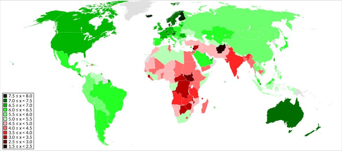
Figure 1: Worldwide Happiness Scores (2022)
Source: World Happiness Report
Figure 2: Happiness Index Trends (1995-2020)
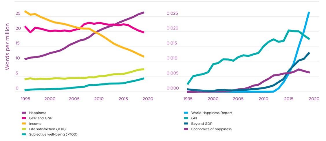
Source: World Happiness Report

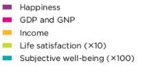
245
Over the years, the World Happiness Report has discovered a multitude of important trends related to global happiness levels. One of the most significant findings trends that was identified by this report is the importance of social connections for overall well-being. This study has consistently shown that those who have strong social ties like family, friends, and colleagues, will tend to report having higher levels of happiness, versus, those who feel more socially isolated and or alone, are more likely to report lower levels of happiness.
In 2021 World Happiness Report found that people's happiness levels have declined over the past year most likely due to the COVID-19 pandemic. However, there are some countries where people have reported higher levels of happiness despite the pandemic. These countries were Finland, Denmark, Switzerland, Iceland and the Netherlands with Finland retaining its position as the world's happiest country for the fourth year consecutively.
The World Happiness Report identifies several other trends related to global wellbeing. For example, countries with stronger social safety nets, such as universal health care and education, tend to be happier. Countries with greater political freedom and stability also tend to be more satisfied. It was also noted that there are many important cultural differences related to happiness. For example, in some cultures happiness is associated with personal achievement and success, while in others it is more closely associated with social connections and community. Understanding these cultural differences is important for policy makers seeking to promote the well-being and well-being of societies. This may also contribute to trends seen in happiness based on location, as counties that are close to each other tend to have similar cultural values. , countries in sub-Saharan Africa tend to be less happy. Understanding these cultural differences can be important for policymakers seeking to promote greater happiness and well-being in their societies.
3.0 LITERATURE REVIEW
The relationship between income and happiness is a longstanding topic of interest in the field of economics. In 1974 Richard Easterling proposed what is now known as the Easterlin Paradox which suggests that there is no relationship between income and happiness past a certain threshold, leading to the income-happiness paradox, which states
246
that despite increasing levels of income happiness levels do not increase. However, future research has challenged this idea by analyzing the relationship between income, education, healthcare, and overall happiness. In this empirical analysis I use six different peer reviewed articles to gain insight into my research.
Both Asadullah et al. (2018), and Hartog and Oosterbeek (2018) both found in their research that there is a link between social comparison and happiness given certain income levels. Asadullah et al. (2018) found that social comparison played a larger role in those with lower incomes, and that the relationship between income and happiness can vary based on one’s demographics. One of the biggest differences seen by demographics was that at lower incomes older individuals and women both reported higher levels of happiness then men with the same income. This is in agreeance with what was found in Hartog and Oosterbeek (2018) research where they found that women and those in rural areas reported lower levels of happiness then men and individuals in more urban areas which suggests that social and environmental factors play more of a role on happiness then income.
Tella and MacCulloch (2008) studied the relationship between income and happiness which suggested that the Easterlin Paradox can be explained by the fact that people tend to compare their income to those around them and not the absolute level of income. This again ties back to research done by Asadullah et al. (2018) because this would give a clear picture as to why men and women at the same level of income would report different levels of happiness and it is because of who they are comparing themselves against. What this work by Tella and MacCulloch (2008) implies is that measuring happiness against an absolute value would not provide and benefit and that by instead measuring happiness at the national level would be able to provide a better understanding of the relationship between income and happiness. Tella and MacCulloch (2008) argued that since individual income may not have a strong relationship to happiness passed a certain threshold, national income may have a stronger effect on overall happiness. The authors propose a concept of "Gross National Happiness" which would consider many factors, for example, social trust, health, and education. From this they were able to find that this measure is positively correlated with national income. This idea of relative or national income was studied again by Hartog and Oosterbeek (2018), what they found was that by digging deeper into their results, they were able to find that relative income, rather
247
than absolute income, is a stronger predictor of happiness, and that individuals with higher relative income tend to report higher levels of happiness. This would mean that using the income of an overall country would not be as beneficial for predicting income as a more localized version of mean income based on location.
In his paper Pugno (2013) explores the ideas of Scitovsky, who was an economist that proposed that happiness is determined not only by absolute income, but also by the relative consumption of goods and services. This topic is later studied again by Van Hoorn and Sent (2016) whose research was on consumerist culture and how it impacts happiness. What they had proposed was that consumer capitalism is the source of happiness, not income in a modern society. This agrees with the ideas from Pugno (2013) that the more we consume, the higher levels of happiness are achieved. The authors, however, do argue that consumer capitalism can create and promote a culture of constant needs for material items and experiences, which can lead to a sense of feeling left out if you do not possess those things All of this can be tied back together with the ideas from Asadullah et al. (2018) where it is all based on demographics.
Some of the policies suggested by these authors include increasing efforts to raise income levels as long as they are accompanied by a measure to change any social factors, since just a boost in income will only lead to a temporary change in happiness levels, Asadullah et al. (2018). Along with this Tella and MacCulloch (2008) also suggest that a policy aimed at promoting overall well-being, and not just increasing individual income, would prove to be more effective in promoting happiness at the national level. What Tella and MacCulloch (2008) suggest as well is that policies aimed at promoting Gross National Happiness may lead to more equitable and sustainable growth. Hartog and Oosterbeek (2018) suggest that a policy in China aimed at reducing income inequality and improving access to resources amongst their people would lead to greater overall happiness. What Pugno (2013) like Hartog and Oosterbeek (2018) states is that policies aimed at reducing income inequality and promoting shared consumption may have positive effects on overall happiness. Pugno (2013) puts these implications on a broader scale then Hartog and Oosterbeek (2018) whose policy implications were only for China. Van Hoorn and Sent (2016) They suggested that a more sustainable and fulfilling approach to happiness would involve a shift towards experiential goods and the cultivation of social relationships.
248
In conclusion, the studies reviewed in this literature review provide valuable insights into the income-happiness paradox and its underlying factors. Going into my analysis I was able to look at the changes suggested by the papers and taking a bigger picture approach to my research and not lasering in only one aspect of the factors that can play an effect on happiness index.
4.0 DATA AND EMPIRICAL METHODOLOGY
4.1 Data
The study uses cross section data from a hundred different countries in 2022. Data was collected from the World Happiness report, Statista and World Population Review. Summary statistics for the data are provided in Table 1.
Table 1 Summary Statistics
Variable Observation Mean Std. Dev. Min Max Happiness Index Score 100 6.132 .804 4.311 7.942 Population (million) 100 2839.231 19693.7 .387 141000 GDP per Capita 100 34324.22 53072.52 368.75 490800 % of population with secondary or more education 100 0.5979 0.2703 0.034 0.974 Education Index 100 0.7244 0.1565 0.298 0.94 Mean Income 100 8871.675 7977.01 369 38874 Average Cost of higher-level education 100 40842.10 44580.19 420.44 180000 Healthcare Index Score 100 73.051 8.974 37.7 86.6 Per capital Healthcare expenditures 100 2035.72 2428.78 20 12318.1 Poverty rate 100 0.22 0.1628 0.002857 0.96 249
4.2 Empirical Model
Following Hartog and Oosterbeek (2018) this study adapted and modified their model Hapi= Ln(MeanIi)+PovRi+GDPi+IndexEi. I have added four new variables to the model
The model could be written as follow:
���������������� = �������� + �������� ���������������� + �������� ������������(�������������������� )���� + �������� ���������������������������� + �������� ������������������������ + �������� ���������������������������� + �������� ������������(��������������������)���� + �������� �������������������� + ����8 ���������������� (1) ���������������� is the happiness index score for country i The happiness index score is found from the happiness index report which is survey data that is aggregated to compute the happiness index score for each country. The happiness index score is a composite measure of different factors that are believed to influence happiness, such as economic well-being, social support, freedom, trust, and generosity. These factors are typically weighted according to their relative importance and combined to create a single score that reflects the overall level of happiness in a country.
Independent variables consist of eight variables obtained from various sources.
Appendix A provides data source, acronyms, descriptions, expected signs, and justifications for using the variables. First, ���������������� represents the percentage of the population in a country with a secondary or higher level of education. ������������(�������������������� )���� is the log value for the average cost of higher-level education in a country. ���������������������������� represents the healthcare index score for a country. ������������������������ is the per capita healthcare expenditures of a country. ���������������������������� is the education index score for each country. ������������(�������������������� )���� is the log measurement of the mean income per capita. �������������������� is the poverty rate of the country and �������� �������� is the GDP per capita of a country.
5.0 EMPIRICAL RESULTS
The empirical estimation results are presented in Table 3. The empirical estimation shows both the positive and negative relationships between the eight independent variables analyzed and the overall happiness score of a country.
250
Table 3: Regression results for the model
p-value gives us a description of how likely it is that the data would have occurred under the null hypothesis of the statistical test
These results represent the output of a linear regression model that examines the relationship between various predictor variables and overall happiness. The model includes nine predictor variables: population with secondary or more education, average cost of higher education, healthcare index score, per capita health expenditures, education index, log mean income, poverty rate, and GDP per capita.
The coefficients table provides estimates of the effects of each predictor variable on happiness, along with their standard errors and significance levels. The coefficients that are statistically significant at the 0.05 level are Log(MeanI), IndexH and CostH. Respectively these represent the log of the mean income for a country, the Healthcare index score and the per capital healthcare expenditure of a country. This indicates that there is strong enough evidence to conclude that these variables have a significant effect on happiness level.
Coefficients Estimate Std. Error T-Value P-Value (Intercept) 1.948e+00 6.805e-01 2.863 0.00521 GDP per Capita -2.798e-07 9.130e-07 -0.307 0.75991 % of population with secondary or more education 8.710e-02 3.201e-01 0.271 0.78676 Education Index 5.848e-01 8.499e-01 0.688 0.49314 Log(Mean Income) 2.379e-01 9.488e-02 2.507 0.01396 Log(Average Cost of higher level education) -1.899e-02 4.179e-02 -0.452 0.65207 Healthcare Index Score 2.217e-02 1.035e-02 2.142 0.03485 Per capital Healthcare expenditures 1.006e-04 2.999e-05 3.355 .00116 Poverty rate 1.289e-01 3.549e-01 0.363 0.71725
251
The residual standard suggests that the model's predictions are within about 42% of the actual happiness scores, on average and the R-squared value of 0.7432 indicates that the predictor variables explain approximately 74.32% of the variability in happiness scores. This r-squared value tells is that there is a strong positive relationship between the model and happiness index score.
Overall, these outcomes suggest that per capita health expenditures, log mean income, and the per capital healthcare expenditures are the most significant predictors of happiness in our model. What this also told us is that population with secondary or more education, average cost of higher education, education index, GDP per capita and poverty rate have little or no significant impact.
These results were not what I was expecting to find. In my initial thesis I predicted that education index, healthcare index and mean income would play the largest roles in happiness score and while the results show that income and healthcare have a significant impact, education doesn’t not have a significant impact on the results.
Some limitations of these results are that the data used is only from 2022, if given the chance to analyze this model over multiple years there could be indicators that other variables also have a significant impact on happiness score. Another limitation is that not all information was available for every country, in my research I had to delete 50 different countries due to missing information which could helped to improve the model even more. In future research I would study this model more historically to see if these same finding held true.
5.0 CONCLUSION
In summary, this empirical analysis highlights the true complexity of the relationship between income, education, healthcare, and happiness. What it suggests is that there is no one simple answer to the Easterlin paradox. The literature review shows that relative income, social comparison, demographic and cultural factors play important roles in shaping the happiness index. This study used cross-sectional data from 100 countries in 2022 to examine and understand the relationship between various indicators and overall well-being. In this study, I modified the model used by Hartog and Oosterbeek (2018) by removing some variables and adding in four new variables to the model. The empirical
252
results indicated positive and negative relationships between the independent variables analyzed and a country’s overall happiness scores. The main outcome shown by the results showed that income and healthcare have a significant positive relationship with happiness score at the 95% confidence level. However, GDP per capita, the proportion of the population with at least secondary education, the education index, and the average cost of tertiary education did not show a significant association with overall satisfaction. Taken together, these results can provide useful insights for policy makers and stakeholders interested in promoting well-being and well-being in different countries. The main policy implication I would suggest would be for countries to increase their healthcare index score which can be improved by also increasing their per capita healthcare expenditure. By improving their overall healthcare policy makers might be able to increase their happiness score. Another policy that can be implemented is an increase in national income. As seen in the literature reviews and the empirical finding, an increase to the mean income can have a significant effect on the well-being of a country’s population. These two in combination can help to bring up many of the scores but of course is not the perfect answer, there are some counties where increasing their budget would not be feasible. This is where I can see education having a bigger impact. If a struggling country is able to get a higher percentage of their population educated, then it can help to grow their country so they can sees an increase in their income and healthcare.
253
Acronym
Appendix A: Variable Description and Data Source
Variable Description
Source
Hap Happiness Index Score
World Happiness Report
IndexH Healthcare Index Score Statista
Index E Education Index score Stasia
CostH Per capita healthcare expenditures per capita Statista
CostE Average cost of higher level education Statista
Mean Income Mean income per capita World population Review
PovR Poverty rate
World Population Review
GDP GDP per capita Happiness Index report
EDU
Proportion of the population with secondary or greater level education
Statista
254
BIBLIOGRAPHY
André van Hoorn & Esther-Mirjam Sent (2016) Consumer Capital as the Source of Happiness: The Missing Economic Theory Underlying the Income-Happiness Paradox, Journal of Economic Issues, 50:4, 984-1002, DOI: 10.1080/00213624.2016.1249746
Asadullah , M. Niaz, et al. “Subjective Well-Being in China, 2005–2010: The Role of Relative Income, Gender, and Location.” China Economic Review, North-Holland, 31 Dec. 2015,
https://www.sciencedirect.com/science/article/pii/S1043951X15001649.
Hartog, Joop, and Hessel Oosterbeek. “Health, Wealth and Happiness: Why Pursue a Higher Education?” Economics of Education Review, Pergamon, 25 Nov. 1998,
https://www.sciencedirect.com/science/article/pii/S0272775797000642.
Paul, S., & Guilbert, D. (2013). Income-happiness paradox in Australia : testing the theories of adaptation and social comparison. Economic Modelling, 30(1), 900-910.
https://doi.org/10.1016/j.econmod.2012.08.034
Pugno, Maurizio, Scitovsky and the Income-Happiness Paradox (December 16, 2011).
University of Cassino, Italy, Department of Economic Sciences, Working Paper No. 7/2011, Available at SSRN: https://ssrn.com/abstract=1973488
Tella, Rafael DI, and Robert MacCulloch. “Gross National Happiness as an Answer to the Easterlin Paradox?” Journal of Development Economics, North-Holland, 29 June 2007,
https://www.sciencedirect.com/science/article/pii/S0304387807000600.
255
Empirical Analysis of NBA 2011 CBA Changes and Their Effects on Competitive Balance.
Derek Smith
Abstract:
This paper investigates the effects of the 2011 collective bargaining agreement on the competitive balance in the National Basketball Association. It illustrates how the different rules and regulations affected various factors within the sport, and in turn how these alterations affected the competitive balance of the NBA. The goal is to exemplify the importance of NBA factors in the competitive balance of the sport and prevent incorrect manipulation of the industry. The results showed that the 2011 CBA did little to none in terms of improving the level of competitive balance within the NBA. All of the factors that were changed by the 2011 CBA countered one another in the efforts to increase competitive balance, however all of these factors showed to be statistically significant towards affecting competitive balance.
JEL Classification: L83
Keywords: Competitive Balance, Regression, Gini, Significance, Coefficient, Standard Deviation
a Student, Bryant University, 1150 Douglas Pike, Smithfield, RI02917. Phone: (207) 468-6998. Email: dsmith29@bryant.edu.
256
The National Basketball Association is one of the more world renown professional sports leagues. The NBA attracts fans from across the globe to watch their favorite players play, and their favorite teams compete for national championships. The concept of competitive balance within sports is measured as the degree in which teams have an equal chance of winning. Competitive balance plays an important role in the success of sports leagues, because without it fans are not as intrigued to watch. The ratification of the new NBA Collective Bargaining Agreement in 2011 was set to increase the luxury tax threshold and rate. The luxury tax threshold is the amount of money that teams can pay players over the salary cap without getting a luxury tax penalty. The rate is the per dollar amount that teams will get penalized if they were to surpass the luxury tax threshold. The agreement decreases the maximum contract length that players can sign from 7 years to 5 years and decreased the percent revenue share between the players and owners to 50%. In the 2011 season alone, there were over two-thirds of the teams in the NBA that were losing money although the league combined was making over four billion dollars in annual revenue. The agreement set out to make teams money again, while increasing competitive balance.
This study aims to enhance understanding of the effects of the 2011 CBA changes in the NBA on competitive balance by providing an empirical analysis of the competitive balance before and after the CBA changes. By conducting this analysis, the study seeks to illustrate the factors that contributed to the changes in competitive balance, and the extent to which the CBA changes in 2011 effected these values. From a policy perspective, this analysis is important because it can evaluate the decisions made in past NBA collective bargaining agreements, in hopes of being more productive in future policies. The findings of this analysis can provide a sort of guidance in evaluating the areas of change that were successful towards competitive balance and areas that could use further improvement.
This paper was guided by the research objective of analyzing all of the given changes that the 2011 CBA implemented into the NBA. The empirical analysis that have been researched offers information on individual variables such as revenue sharing or
1.0
INTRODUCTION
257
salary cap and how they affect competitive balance. This paper offers the full layout to illustrate how all variables interact with each other and what variables should be more focused on.
The rest of the paper is organized as follows: Section 2 is the trend of the given topic. Section 3 is the literature review. Section 4 is the data and empirical methodology. Section 5 is the results and section 6 is the conclusion.
2.0 TREND
There are multiple ways in which competitive balance can be measured in sports. The Gini Coefficient of wins and the Standard Deviation of wins were the two that I used in my models to assess the effects of the 2011 CBA changes on competitive balance. Figure 1 shows the values of these two measurements over the past 20 years in the NBA.
Figure 1: Measures of Competitive Balance
As shown in Figure 1, there has been no significant change in the level of competitive balance from 10 years before the 2011 CBA changes and 10 years after. The standard deviation of wins was slightly decreasing before 2011 then began to slightly increase after 2011. The Gini coefficient of the wins stayed relatively the same over the past 20 years in the NBA.
0 0.2 0.4 0.6 0.8 2001 2002 2003 2004 2005 2006 2007 2008 2009 2010 2011 2012 2013 2014 2015 2016 2017 2018 2019 2020 2021 Season Gini SD Wins 258
In Figure 2, there is a clear trend between Player Revenue Share and Salary Cap. When the NBA Players Association and the team owners come together to create Collective Bargaining Agreements, the primary goal is to ensure the league is an efficient and healthy industry. The negative trend line between Salary Cap and Player Revenue Share tells a slightly different story. The Salary Cap variable naturally increases as teams make more money. The more money teams have, the more capable they are of paying their players. As shown, when the Salary Cap increases, the Player Revenue Share decreases. This means that owners are taking advantage of the changes in the CBA agreements and taking a higher percentage of the revenue as more money flows in.

 Figure 2: Salary Cap and Player Revenue Share
48 49 50 51 52 53 54 55 56 57 58 59 0 0.2 0.4 0.6 0.8 1 1.2 Player Revenue Share Salary Cap 259
Figure 3: NBA Attendance
Source: HoopHype Website
Figure 3 illustrates the total NBA game attendance from the year 2001-2018. The years 2018 to 2021 were taken out of consideration due to the COVID-19 pandemic. As shown, there has not been a significant increase or decrease in NBA attendance over the past 20 years. There was a decrease in attendance for a minimum amount of time from 2011 to 2013, around the time where the 2011 CBA was put into place. The per yer attendance behaves similarly to that of the levels of competitive balance. There has been little to no change in either. This suggests that they move in the same way, and if competitive balance were to change, the fans would become more or less interested in watching the NBA depending on the level in which the competitive balance changes, and the attendance numbers would reflect that.
3.0 LITERATURE REVIEW
The National Basketball Association is a world renown competitive sports league that takes place in the United States. The stability and structure of the financials within the sport, along with the relations with the players, is built upon the Collective Bargaining Agreement (CBA). The CBA pairs with the National Basketball Association (NBPA) to cover the terms and conditions for the overall employment and well-being of the players. Every few years, the CBA is refreshed to keep up with problems that may
0 5 10 15 20 25 2001 2002 2003 2004 2005 2006 2007 2008 2009 2010 2011 2012 2013 2014 2015 2016 2017 2018 Attendance Millions Season 260
arise within the sport. In 2011, there were significant changes in the CBA that would primarily target the concerns on competitive balance. There have been various empirical studies that illustrate the effectiveness of different variables on competitive balance.
Colby and Jenkins (2016) found that revenue sharing within a league can increase the amount of resources that small market teams have, and therefore decrease the amount of competitive imbalance between sports. They found that when revenue disparities in Major League Baseball were solved, the competitive balance was more equal. Looking at other sports like the MLB, Kesenne (2004) looked at three different sports when analyzing revenue sharing. Kesenne (2004) found that up to a certain point, revenue sharing increases competitive balance. After that point, it starts to negatively affect the sport and decrease competitive balance.
There are a wide range of variables that the 2011 CBA looked to alter in hopes of increasing competitive balance other than revenue sharing. The 2011 CBA had completely revamped the way in which teams were to pay for their luxury tax, almost disincentivizing teams to go over this tax and therefore wouldn’t spend more money on players. Grant and Shorin (2017) studied the impact of the NBA luxury tax and found no significant effect on competitive balance, showing that it is perhaps an ineffective tool when trying to increase the competitive balance within a sport.
Like this empirical analysis, Totty and Owens (2011) examined the effects of salary caps on competitive balance and found that it may not only be ineffective but may negatively impact competitive balance within sports. They used the standard deviation of wins as the independent variable, similar to that of this analysis. Couture (2016) also analyzed the effects of salary cap and competitive balance, specifically in the NBA. This analysis used the 1998 CBA to analyze the changes in competitive balance, and it was found to be a big impact on the increase in such. All empirical papers studied , including Totty and Owens (2011), Couture (2016) and also Alwell (2020) used Standard Deviation of Wins as their dependent variable and their form of measurement for competitive balance.
261
4.0 DATA AND EMPIRICAL METHODOLOGY 4.1 Data
The study uses annual time series data. Data was obtained from the HoopsHype and TeamRankings websites, as well as other articles such as NBA revenue statistics (2001-2022) by Dimitrije Curcic. Summary statistics for the data are provided in Table 1.
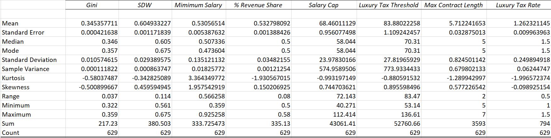
The Gini Coefficient was one of the two independent variables that I used for the measurements of competitive balance. The Gini Coefficient considers the equality of the distribution of wins amongst NBA teams. I used the equation G = (2 / n(n-1) * mu) * Σ[i=1 to n](i * xi) - (n + 1) / (n - 1) to calculate the observed values for each year in the NBA 10 years before and after the 2011 CBA. The n equals the number of teams in the NBA, mu is the mean number of wins per team, xi is the number of wins for team 1 and the Greek uppercase letter sigma means the sum of all the values of i multiplied by xi ranging from team 1 to n.
The other independent variable used for measuring competitive balance is the standard deviation of wins, which considers the amount of variation between wins amongst the NBA teams for every season from 2001-2021. The equation used was σ = sqrt[Σ(xi - mu)² / (n - 1)]. The square root of the variance of the residuals was taken for both regression models to indicate the absolute fit of the models to the data.
Table 1: Summary Statistics
262
Table 2: Correlation Coefficient
Table 2 shows the correlation coefficient of the data used. There were only a few significant correlations between all the variables. There was a high correlation between Salary Cap and Luxury Tax Threshold at .988. As the Salary Cap increases, there is naturally an increase in the threshold of the Luxury Tax. There was also a high correlation between Max Contract Length and Luxury Tax Rate. There were a few others, but most were not significantly correlated, eliminating the risk of multicollinearity. This allowed the individual variables to be interpreted as contributing in their own ways.

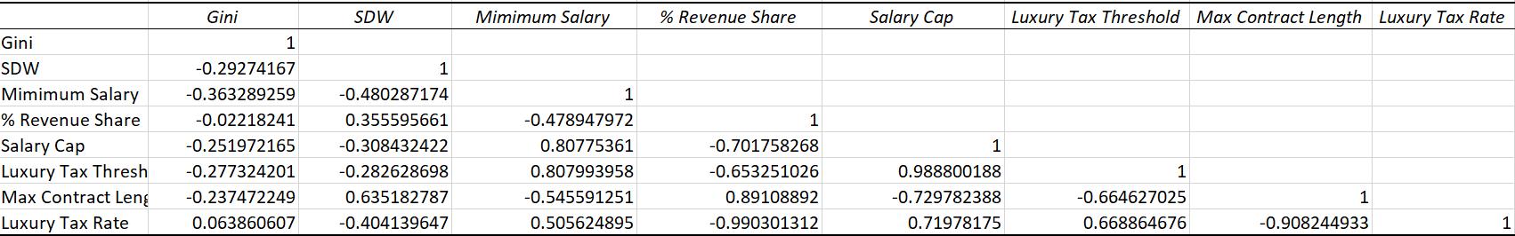
4.2 Empirical Model
The models could be written as follows:
Model 1:
Model 2:
The models are almost completely identical other than the dependent variables of Gini and SDW. These differences were to illustrate how the independent variables affected various measures of competitive balance.

263
Independent variables consist of seven variables obtained from various sources. Appendix A provide data source, acronyms, descriptions, expected signs, and justifications for using the variables. First, ���������������������������������������������������� represents the minimum amount of money a player can sign for each year. %��������������������������������ℎ������������ is the percentage of revenue that the individual team makes that is shared with the players that formulate the team. ������������������������������������ is the total amount of money that teams can sign players for in each season.
����������������������������������������ℎ������������ℎ������������ is the amount of money that teams can exceed the Salary Cap by before enduring a luxury tax penalty. MaxContractLength is the maximum number of years that a player can sign for in a contract. LuxuryTaxRate is the per dollar amount that teams will be penalized once exceeding the luxury tax threshold. The independent variables differed in whether or not they were directly changed by the 2011 CBA. For example, SalaryCap and MinimumSalary are variables that were not changed by the CBA. These variables are progressively changing due to the environment of the economy. Variables such as either or the luxury tax variables, or MaxContractLength, were directly affected. The combination of both types of independent variables allowed for the results to show which factors truly are significant towards affecting the level of competitive balance.
5.0 EMPIRICAL RESULTS
The empirical estimation results are presented in Table 2. The empirical estimation shows that all seven of the independent variables used were statistically significant towards determining the level of competitive balance in the NBA at the 1%, 5% and 10% levels. The signs of the coefficients for every variable except for minimum salary were the opposite between the two models. This is expected due to the nature in which both independent variables are calculated. The key commonality between both models was the differing signs of the coefficients within the respected models. Both models have all of the independent variables opposing one another in regard to how each variable individually affected the value of the competitive balance.
264
Model 1 and 2 both had high R2 values, indicating that both fit the model well. The root mean squared error was tested to ensure the high performance of the models by comparing the observed vs. predicted values.
Note: *** , **, and * denotes significance at the 1%, 5%, and 10% respectively. Standard errors in parentheses
Competitive Balance I Gini II SDW CONSTANT -.0132 (.0339) 1.082 (.0695) MinimumSalary - .042*** (.002) -.134*** (.005) %RevenueShare .775*** (.046) -1.34*** (.095) SalaryCap -.001*** (.000008) .003*** (.0001) LuxuryTaxThreshol d .0008*** (.000006) -.0002*** (.0001) MaxContractLength - .020*** (.0007) .0635*** (.0014) LuxuyTaxRate .079*** (.007) -.098*** (.0143) R2 0.733 0.855 F-statistics 285.7*** 613.97*** Number of obs. 628 628
Table 2: Regression results for the ASEAN-5
265
A couple of findings were consistent to the major empirical studies that were analyzed to inspire the models created. Like that of Louchheim (2018), luxury tax rate was significant towards affecting the level of competitive balance. Paultor (2010), although studying the NFL and MLB, found similarities in that the revenue affects the level of competitive balance of a sport. The variable %RevenueShare was found to be statistically significant for both models, as well as MinimumSalary and SalaryCap. These findings are consistent with Totty and Owens (2011).
Interpreting these results begins with recognizing that all of the explanatory variables interacted in opposite directions of one another. This indicates that while some of the factors that were changed in the 2011 Collective Bargaining Agreement positively affected competitive balance, others did not. The policymakers tried to change too many different factors, and this resulted in multiple affects countering one another and the efficiency towards higher competitive balance was limited.
6.0 CONCLUSION
In summary, the changes made in the 2011 Collective Bargaining Agreement, which included increased luxury tax threshold and rate as well as decreased maximum contract length and percent revenue share, made no significant change to the competitive balance of the NBA. In studying multiple methodologies towards measuring competitive balance, through empirical modeling I was able to determine that all explanatory variables used are statistically significant towards affecting competitive balance. Furthermore, I was able to determine that many of these factors countered one another.
The policy implications of the study are that policy makers, in this case NBA owners and the Players’ Association, need to carefully evaluate the potential effects that certain changes may have. Specifically, they should focus more of their attention on factors that positively affect competitive balance, like minimum salary and salary cap. One limitation of the study was not accounting for other factors such as coaching and team strategy, that may also influence competitive balance.
266
This study contributed to the extant literature by empirically analyzing the links between multiple factors that were changed by the 2011 CBA and competitive balance. Using two alternative measures of competitive balance, I empirically accessed the effects that the 2011 CBA changes made to competitive balance. The results showed that there are an extensive number of variables that are significant towards competitive balance, and the different affects that the individual factor changes had led to little to no progress in the level of competitive balance in the NBA.
Appendix A: Variable Description
Acronym Description
MinimumSalary
The minimum amount of money that a player can sign for on a per year salary
%RevenueShare
The percent of the revenue that NBA teams are required to share with their players
SalaryCap
The maximum amount of money a team can spend on players in each season
LuxuryTaxThreshold Distance as crow fly from Washington DC to the host country capital city
MaxContractLength The maximum number of years a player can sign for in a given contract
267
The per dollar amount that teams are taxed once they surpass the luxury tax threshold.
LuxuryTaxRate
268
BIBLIOGRAPHY
Alwell, Kevin. “Analyzing Competitive Balance in Professional Sport.” (2020)
Couture, Cody. “Salary Caps and Competitive Balance in the NBA.” (2016).
KÉsenne, S. (2004). Competitive Balance and Revenue Sharing: When Rich Clubs Have Poor Teams. Journal of Sports Economics, 5(2), 206–212.
Louchheim, Benjamin. “Luxury Tax and Competitive Balance in the NBA.”(2018)
Paulter, Matt. “The Relationship Between Competitive Balance and Revenue win America;s Two Largest Sports Leagues.” (2010)
Shorin, Grant. “Team Payroll vs. Performance in Professional Sports: Is Increased Spending Associated with Greater Success.” (2017)
Totty, Evan, and Mark Owens. “Salary Caps and Competitive Balance in Professional Sports Leagues.” Journal for Economic Educators, Middle Tennessee State University, Business and Economic Research Center, 1 Jan. 1970
269
Granger Causality Test for Agricultural Production to Economic Growth in Thailand
Joshua Soares
Abstract:
This study will dive into looking at the relationship of GDP growth and agricultural production in Thailand. In order to complete this study, we will use a Unit Root test, a Johanson Cointegration Test, a Granger Causality test, and finally an Impulse response function. The results will be able to show us whether or not there is a causal relationship between agricultural production and GDP growth. The results of the tests showed us that our only variable that had any significance was Thailand’s Net Trade.
JEL Classification: Q10, Q15, Q17, Q19
Keywords: Agricultural Production, Economic Growth, Thailand.
a Department of Economics, Bryant University, 1150 Douglas Pike, Smithfield, RI02917.
Email: Jsoares9@bryant.edu
270
1.0 INTRODUCTION
The agricultural sector in Thailand takes up about one third of the countries labor force while only taking up about six percent of the countries GDP. This is just a perfect example of the sector not working at its full potential which has been concerning poicly makers for years. Within this study we are going to be looking for the biggest factors of the agricultural sector that have a significant impact on the countries GDP growth. We’re going to be looking at the direction and the intensity of a causal relationship, if there is one. Were going to use multiple tests to look at this, including the Granger Causality Test, an impulse response analyses, a unit root test and then a Johansen Cointegration test. Many years ago in Thailand, agriculture was a significant contributor to the countries economic. Thailand’s location, their weather, and the ground they plant in make it a perfect place to grow crops and have an agriculturally backed economy. This sector employs a good number of the labor force in Thailand. Over sixteen million people are working in agriculture which makes it the highest employed sector in Thailand. However even though it is such a contributor to the country’s employment, the contribution to the country’s GDP has been declining. In the 1960s, the agriculture sector took up almost forty percent of Thailand's GDP. However, this figure has since steadily been on the decline. Today it only accounts for only about 6% of the country's GDP. This decline can be attributed to several factors. The demand for Thai agricultural products like rice is on the downfall. Also, climate change and some supply chain issues as well.
The primary objective of this paper is to find out the key determinants of GDP growth that are within the agricultural sector of Thailand. We will need to investigate into whether or not
271
there is a causal relationship between agricultural production and economic growth, and if there is one, also to find out the direction and strength of this relationship.
To identify the key determinants of GDP growth within the agricultural sector of Thailand, we will employ a number of economic tests To start we are going to use a unit root test to find out if the time series data is stationary or not. If it is not stationary, we will have to employ appropriate changes to make it stationary. Secondly, we are going to be using a Johansen Cointegration Test in order to see if there is a long-term relationship of agricultural production and GDP growth. This test shows us the strength and the direction of any possible relationships. The third test we are going to use is called the Granger Causality Test which looks at if there is a causal relationship between agricultural productivity and GDP growth. This also looks at the direction of the relationship and whether or not there is a causal one. Lastly, we’ll use an Impulse Response function to look at the dynamics of any existing relationship between each independent variable and the dependant.
2.0 TREND
Figure 1 shows the growth of GDP from the agricultural sector in Thailand in 2020 to 2022 with a forecast for 2023. It shows an obvious decrease in 2020 due to Covid-19. It shows the small share over the passed few years however a predicted increase for the 2023 year.
272
In Thailand, the agricultural sector has been a big contributor to their economy for years. But over the past decade, the sector’s productivity has declined as far as its contribution to the country’s GDP growth. The largest growth rate over past ten years was in 2011 when the sector’s contribution to GDP only grew by about 15%. The lowest was recorded in 2020 during the pandemic with a decrease by about 6%.
The overall trend of GDP growth from the agriculture sector in Thailand has been declining over the last decade. The average growth rate dropped from around 5% in 2010 to less than 1% in 2020. This trend shows the challenges that the agricultural sector has faced in recent years. Factors such as the declining demand for traditional Thai agricultural products and the impact of climate change on agricultural production. The sector's share of GDP dropped from
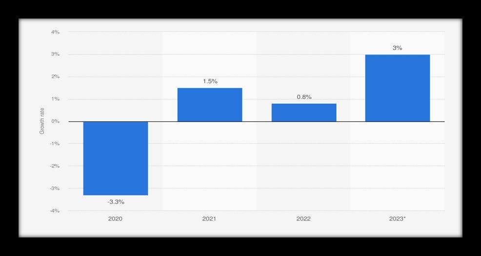 Figure 1: The Growth of GDP from agriculture sector from Thailand in 2020 to 2022 with a forecast for 2023
Source: OAE Statista 2023
Figure 1: The Growth of GDP from agriculture sector from Thailand in 2020 to 2022 with a forecast for 2023
Source: OAE Statista 2023
273
around 10% in 2010 to less than 7% in 2020. This decline further shows the need for policymakers to implement measures that can promote agricultural development and increase the sector's contribution to the country's GDP.
As well as all over the world, Covid 19 had a strong negative impact on the agricultural sector in Thailand. During this time, the sector’s contribution to the countries GDP shrunk by about six percent, due to all the disruptions within the supply chain. This just goes to show that there needs to be improvements on the resilience of the sector in order to bounce back from problems like the pandemic.
The agriculture sector in Thailand has been facing various challenges over recent years, which lead to a declining trend in its GDP growth rate and contribution to the country's overall GDP. However, with appropriate policy changes, such as improving productivity and competitiveness, enhancing supply chain resilience, and focusing on specific sectors within the whole agricultural sector, it can recover and begin to contribute much more to Thailand's economic growth over the next few years.
3.0 LITERATURE REVIEW
Productivity in the agricultural sector has been seen having a positive impact on the economic growth of many developing countries. (Nahanga and Bečvářová, 2015; Güzel and Akin, 2021; Chandio et al., 2015). In Nigeria for example, the exports from the agricultural sector have been shown to have a positive impact on economic growth. (Nahanga and Bečvářová, 2015). Although the sector’s contribution as a whole depends on the smaller more specific subsector’s productivity because some have more of an impact than others. (Chandio et al., 2015). Policymakers should focus on enhancing the productivity and efficiency of specific
274
sub-sectors to maximize the overall contribution of the agricultural sector to economic growth. The levels of quality of the institutions within the sector have been proven to be linked to positive economic expansion. (Blonigen, 2005; Busse and Hefeker, 2005). Policymakers should be working on improving the institutional quality across the sector in order to attract investment and be able to promote economic growth. Inflation also has a significant impact on the economic performance and the farming sector (Lins and Duncan, 1980). This shows us how important it is for macroeconomic stability among agricultural production.
The relationship between land tenure systems and agricultural productivity has been found to be a major barrier to higher output from the sector, (Yano, 1968). This shows the importance of providing secure land tenure to farmers to promote agricultural production and economic growth. Agricultural sector can play a crucial role in promoting economic growth in developing countries. Policymakers should focus on enhancing the productivity and efficiency of specific sub-sectors, improving institutional quality, ensuring macroeconomic stability, and providing secure land tenure to farmers to maximize the sector's contribution to economic growth.
4.0 DATA AND EMPIRICAL METHODOLOGY
4.1 Data
In this study, we used data from the World Development Indicators to investigate the relationship between the production levels of the agricultural sector and economic growth in Thailand. The time series data that was used in this study was from the years 1985 up to 2021 which allowed the study to look at some of the long term relationships and trends of agriculture’s effect on economic expansion.
275
The empirical methodology is based on a similar study titled "The role of agricultural productivity in economic growth in middle-income countries: An empirical investigation" by Arif Eser Güzel and Cemil Serhat Akin. The model used in this study is specified as follows:
The dependent variable, GDP per capita, is measured in constant 2010 US dollars. The independent variables include agricultural productivity (AGRI), gross capital formation as a percentage share of GDP (GCF), human capital as the average years of schooling and rate of return to education (HC), and trade openness as the sum of total exports and total imports as a percentage share of GDP (TRD).
Below are the two tests that are used as my summary statistics. I used a Unit root Test, as well as a Johanson Cointegration Test.
1 Unit Root Test
Method Statistic Prob. ** CrossSections Obs Null: Unit Root (assumes common unit root process) Levin, Lin & Chu t* -0.65826 0.255 6 213 Null: Unit Root (assumes individual unit root process) Im, Pesaran and Shin W-stat -1.06753 0.1429 6 213 ADF – Fisher Chi-square 21.2740 0.0465 6 213 PP – Fisher Chi-square 22.0137 0.0374 6 213 276
2 Johanson Cointegration Test
4.2 Empirical Model
However, in this study, we modify the model to better suit the specific characteristics of the Thai economy. Our modified model includes the following independent variables:
i=1: INFLR - Inflation rate
i=2: AGEXP – Agricultural product exports as a percentage of total exports
i=3: AFF - Agricultural Forestry and Fishing
i=4: AGLAND - Agricultural land area in square kilometers
i=5: NETTRADE - Net trade
With my model looking like this:
5.0 EMPIRICAL RESULTS
Unrestricted Cointegration Rank Test (Trace) Hypothesized Trace 0.05 No. of CE(s) Eigenvalue Statistic Critical Val. Prob. ** None * 0.681077 121.0288 95.75366 0.0003 At most 1* 0.639323 81.03056 69.81889 0.0049 At most 2 0.417081 45.33853 47.85613 0.0846 At most 3 0.319948 26.44879 29.79707 0.1159 At most 4 0.306753 12.95326 15.49471 0.1165 At most 5 0.003718 0.130371 3.841465 0.7180
Table
Null Hypothesis Obs F-Statistic Prob. GDP does not Granger Cause AG_EXPORTS 35 0.30542 0.7391 AG_EXPORTS does not Granger Cause GDP 0.24602 0.7835 GDP does not Granger Cause INFLATION_RATE 35 1.05398 0.3611 277
2: Granger Causality Test
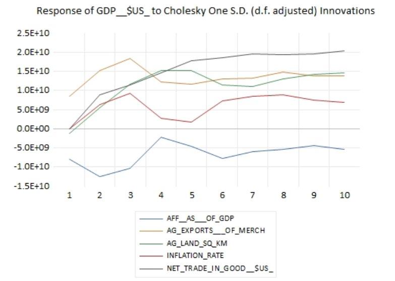
INFLATION_RATE does not Granger Cause GDP 3.02153 0.0638 GDP does not Granger Cause NET_TRADE_ 35 3.99821 0.0289 NET_TRADE_ does not Granger Cause GDP 5.72427 0.0078 GDP _ does not Granger Cause AFF 35 0.42429 0.6581 AFF__ does not Granger Cause GDP 0.00253 0.9975 GDP does not Granger Cause AG_LAND_ 35 2.02583 0.1495 AG_LAND_ does not Granger Cause GDP__$US_ 2.19309 0.1291
278
Table 3: Impulse Response Function
The findings of the empirical analysis are presented by Tables 2 and Table 3. Table 2 shows us the findings from the Granger Causality test, that looked at the causal relationship between GDP per capita, and all of the independent variables individually. The results show that Agricultural product exports as a percentage of merchandise exports, inflation rate, agriculture/forestry/fishing, and agricultural land area do not have a causal relationship with GDP per capita. However, net trade does have a statistically significant causal effect on GDP per capita at the 5% significance level.
Table 3 shows the impulse response function for all of the variables that were included in the model. What this test does is measure the effect on the variables for a one standard deviation shock to each of the independent variables to the dependent over time in both the short tun and the long run. The results show us that a shock to net trade has a positive and significant effect on GDP per capita in the short run, but over time the effect drifts away. On the other hand, a shock to agricultural land area has a negative effect on GDP per capita in the short run, but overtime, the effect then turns positive and significant in the long run.
Overall, our results from the test show us that net trade is the only independent variable that has a causal relationship with economic growth. The findings also show us that the amount of agricultural land has a negative effect on GDP growth in the short run, however in the long run, there is a positive effect. These findings have important implications for policymakers in Thailand, who may need to consider the effects of net trade in goods and agricultural land use on economic growth when designing development strategies.
Going forward, looking at some policy implications, Thailand really needs to hone in on the more specific subsectors of the agricultural sector. The country needs to make policies that
279
are not too broad when looking at the agricultural productivity levels and how to increase them. Based off of the results from this study, policymakers in Thailand need to be focusing on increasing the amount of agricultural exports as we have seen that net trade has a significant effect on GDP growth. They also need to be setting aside more land for agriculture use in order to increase the sectors productivity in the long run.
Saying that, in this study the independent variables should have been more specific in order to have had more statistically significant variables as well as more variables that had a legitimate causal relationship with GDP growth. This would have allowed for more specific policy implication suggestions from this study.
5.0 CONCLUSION
This study aimed to examine the impact of different sub-sectors of the Agricultural sector on Thailand's GDP. The results suggest that not all sub-sectors of agriculture affect GDP equally. Specifically, the impulse response graph showed that AFF has a negative effect on GDP, while net trade and land have a positive effect. These findings suggest that a broad approach to increasing agricultural production may not be as effective in boosting GDP as a more precise plan focused on increasing agricultural land and exports. This study supports previous research that indicates that focusing on agricultural exports and land development could be more beneficial for Thailand. Currently, the Agricultural sector accounts for only 6% of Thailand's GDP, even while it employs one-third of the country's labor force. The overall trend of GDP growth from the Agricultural sector has been decreasing over
280
the past ten years. Therefore, it is crucial to narrow the focus on specific aspects of Agriculture that have a more significant impact on GDP.
The independent variables analyzed in this study included the inflation rate, Agricultural Exports, AFF, Agricultural land, and Net Trade, with Net Trade being the most statistically significant. Therefore, this study suggests that Thailand should prioritize agricultural exports and land development in its agricultural sector policies to boost the country's GDP. Future research could examine the impact of other factors, such as technological advancements, on the Agricultural sector's growth in Thailand.
281
APPENDIX
GDP Gross Domestic Product measured in constant US dollars
AFF Agriculture Forestry and Fishing
AG-LAND Agricultural land – available arable land measured in square kilometers
AGEXP Agricultural exports as a percent of merchandise exports
INFLR Inflation Rate measured as CPI
NETRD Annual Net Trade
282
BIBLIOGRAPHY
1. Güzel, A. E., & Akin, C. S. (n.d.). The role of agricultural productivity in economic growth in middle-income countries: An empirical investigation. Department of Economics, Hatay Mustafa Kemal University, Hatay, Turkey.
2. Chandio, A. A., Yuansheng, J., Rahman, T., & Khan, M. N. (2015). Analysis of agricultural sub-sectors contribution growth rate in the agriculture GDP growth rate of Pakistan.
3. Verter, N. (n.d.). THE IMPACT OF AGRICULTURAL EXPORTS ON ECONOMIC GROWTH IN NIGERIA.
4. Yano, T. (1968). Land tenure in Thailand. Asian Survey, 8(10), 853-863. doi: 10.2307/2642391.
5. Johnson, D. G. (1980). Inflation, agricultural output, and productivity. American Journal of Agricultural Economics, 62(5), 917-923. doi: 10.2307/1240328.
6. Aye, G. C., & Odhiambo, N. M. (n.d.). Threshold Effect of Inflation on Agricultural Growth: Evidence from Developing Countries. Department of Economics, University of South Africa, Pretoria, South Africa.
7. U.S. Department of Commerce. (2021). Thailand - Agriculture. Country Commercial Guides.
8. United Nations Thailand. (2021, March 30). Thai agricultural sector: Problems & Solutions.
283
9. Statista. (2021). Agriculture in Thailand - statistics & facts.
10. Encyclopedia Britannica. (n.d.). Thailand - Agriculture, forestry, and fishing. In Encyclopedia Britannica.
284
A Granger Causality Test on the Misery Index Effects on Domestic Violence
Talia Vicentea
Abstract
This paper investigates the possibility of an increase in domestic violence because of high inflation and unemployment rates in the United States. Inflation and unemployment are two factors that add together to contribute to the Misery Index. This index was created in 1970 by Arthur Okan, who used the index as a measure of economic distress felt by everyday people, due to the risk of, or actual, joblessness combined with an increasing cost of living. The data is collected from 1950’s to 2019 on factors such as unemployment, inflation, poverty, education, and GDP per capita. The results show that an increase in the misery index causes an increase in domestic violence.
JEL Classification: C12, E31, K4
Keywords: Misery Index, Crime.
a Department of Economics, Bryant University, 1150 Douglas Pike, Smithfield, RI02917. Phone: (401) 232-6379. Email: tvicente1@bryant.edu.
285
1.0 INTRODUCTION
The Misery Index has been used to study the effects of a variety of variables, such as unemployment and inflation on crime, political election results, weight loss, and happiness. Looking at not only the various areas across the United States, but also on a global scale. This study aims to enhance understanding on the Misery Index effect on domestic violence as annually, 10 million men and women are domestically abused by their partner (National Statistics, 2023). From a policy perspective, this analysis is important because it allows them to focus their attention on geographic areas that have low GDP and high inflation within the United States, and can implement economic policy to control inflation rates, while trying to increase GDP to decrease the amount of domestic violence year to year in the United States. The relevance of this study is that it looks at domestic violence on a national level year to year, to evaluate what the correlation is of having a high inflation rate, low education, low GDP, high poverty, contributes to higher levels of domestic violence within intimate partner relationships. While the Misery Index is an economic tool that can be used to look at macroeconomic issues, it cannot directly look at social issues like domestic violence, or overall violence as a sole indicator of correlation. Even though historically, an increase in the Misery Index is shown to be linked to an increase in overall violence, from economic distress, other social factors affect the rate of domestic violence. Yet, an increase of inflation and unemployment can exacerbate the issue of domestic violence. As an increase in Misery can cause financial stress, unemployment, limited resources, mental health problems, and social isolations.
This study aims to investigate whether or not Saboor et al. (2016) thesis, that domestic country face more of a long run effect on domestic violence, was the same conclusion for a country like Pakistan, as it is in the United States. While utilizing annual data from the year 1965-2020, there was shown causality between inflation and the effect of domestic violence in the long run. In the short run, both inflation and GDP contribute to domestic violence. This result was found from running a unit root, Johansson cointegration, and Granger Causality test.
286
This paper was guided by three research objectives that differ from other studies:
First, it investigates the possibility of interdependence between domestic violence and the Misery Index. Second, it incorporates the Misery Index into a model to exam how the independent variables of poverty, GDP, inflation, and education affect domestic violence levels. Last, it analyzes the misery index on domestic violence using a panel data model. The rest of the paper is organized as follows: Section two gives a brief literature review. Section three outlines the empirical model. Data and estimation methodology are discussed in section four. Finally, section five presents and discusses the empirical results. This is followed by a conclusion in section six.
287
2.0 TREND of Misery and Domestic Violence
Figure 1 shows in the inflation rate from 1965 to 2020 for the United States. Inflation is measured in this instance by the cost of consumer prices. The consumer price index (CPI) is a basket of goods such as food, housing, transportation, and recreation, that shows the average cost of goods for that period. The inflation rates have hit peaks and troughs over the past 60+ years.
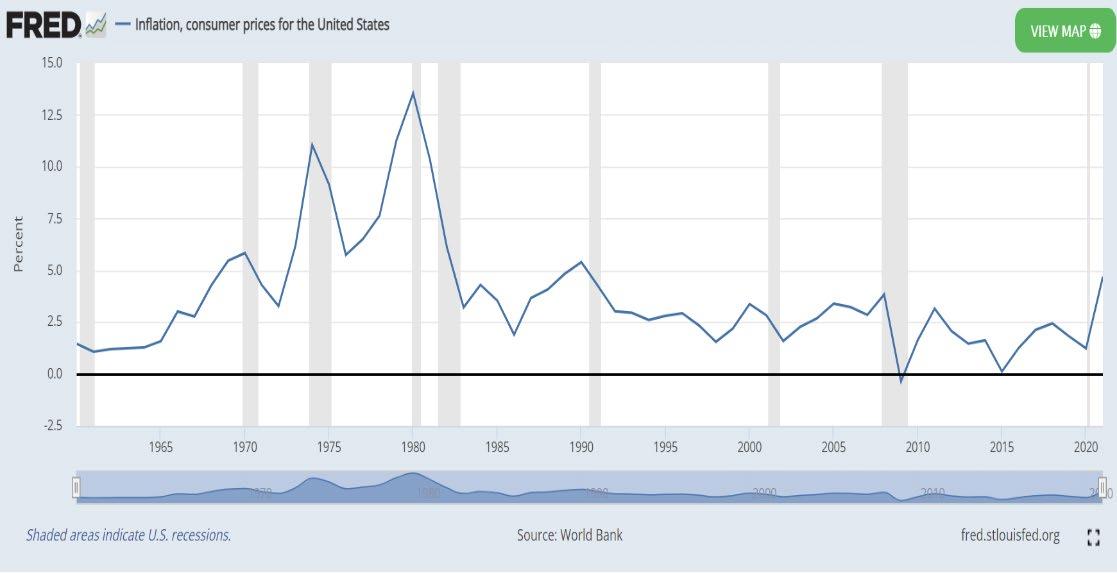 Figure 1: Inflation, consumer prices for the United States
288
Source: FRED, World Bank
Figure 2 shows the United States’ unemployment rate from 1960 to 2020. Unemployment and inflation are added together to create the Misery Index. In 202 Unemployment hit a record breaking 60 years high, even during the 2008-2009 recession, the percentage of US citizens unemployed never came close to the 15% level it reached in 2020 due to COVID19. This effect may have had a strong correlation to the level of domestic violence as the Misery Index also accounted for growing inflation.
Figure 2: United States Unemployment Rate
Source: FRED, US Bureau of Labor Statistics
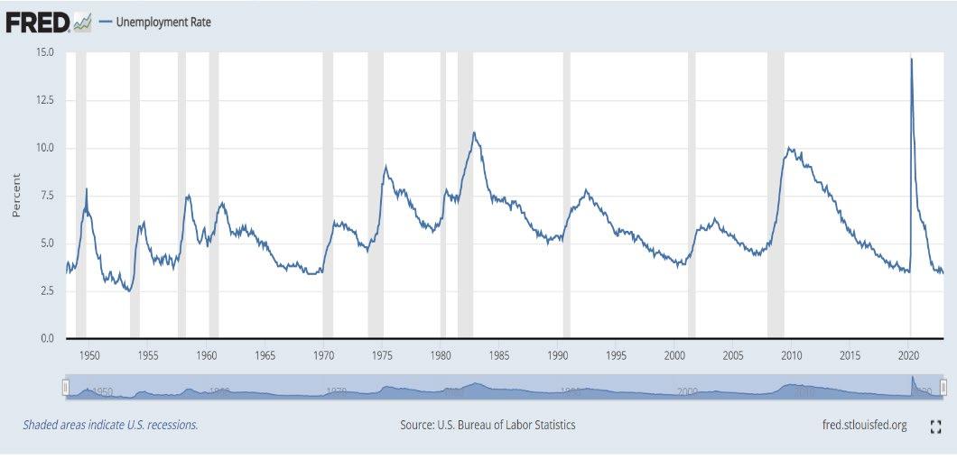
289
Figure 3 shows the rate of domestic violence victimizations by crime type. The data is based on a change from 1993 to 2021, either having an increase, decrease, or no change in domestic violence during the past thirty years. Violent victimization, rape, assault, robbery, and theft have all had a decrease. Violent victimization decreased over 60%. Despite 2020 having a major economic crisis, with high rates of inflation and unemployment, the level of crime compared to 1993, during the start of the Tech Bubble, was still higher in 1990’s compared to present levels of crime.
Source: Bureau of Justice Statistics
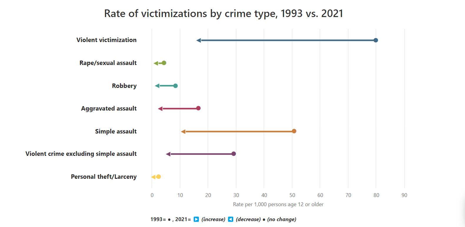 Figure 3: Rate of Victimizations by Crime Type, 1993 vs 2021
290
Figure 4 shows the Misery Index based on unemployment rate and consumer price index for all urban consumers. All items are from a US city average. The Consumer Price Index for All Urban Consumers: All Items is a price index of a basket of goods and services paid by urban consumers. Percent changes in the price index measure the inflation rate between any two time periods. The most common inflation metric is the percent change from one year ago. It can also represent the buying habits of urban consumers. This index includes roughly 88 percent of the total population, accounting for wage earners, clerical workers, technical workers, self-employed, short-term workers, unemployed, retirees, and those not in the labor force.
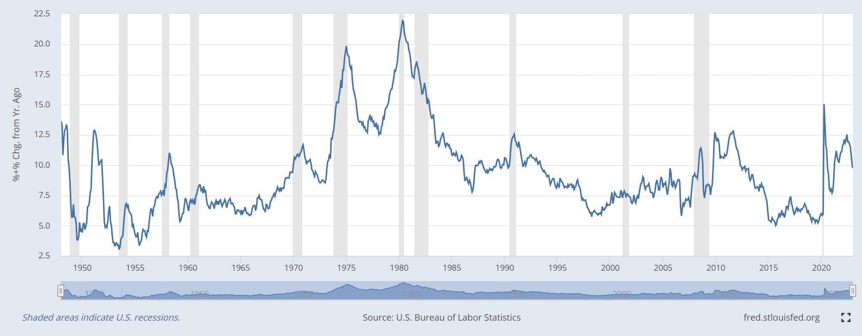 Figure 4: Misery Index 1960 to 2023
291
Source: FRED, Bureau of Labor Statistics
3.0 LITERATURE REVIEW
In a study by Açcı and Çuhadar(2021), it was found that crime has historically been a subject matter for social sciences. Economics has begun its study on crime starting with a person’s intensity to commit crime based on microeconomic theories, however, in recent years the misery index has linked crime to inflation and unemployment rates. The model used the prison population per 100,000 inhabitants as the dependent variable, and the misery index, GDP, poverty, and education for the independent variables in the model. Data from the World Bank, UNDP, University of Oxford, and UNODC helped create a reliable data set. This study analyzed the ‘Fragile Five’ in relation to the misery index, that is Indonesia, Turkey, Brazil, India, and South Africa. It was found that increases of the misery index from 2004-2017 have increased crime. Research on the Misery Index has been used to track crime rates in various countries. In Nigeria, institutional quality, from government, and laws, was found to reduce crime rates in the short term in Nigeria, however long-term economic misery was shown to have an increase in crime. Connecting the social sciences, which advocate for government reforms for developing countries to be able to create more peaceful conditions for citizens in various countries. It was also established in this study that democratic nations such as Nigeria, were subject to more fluctuation in crime rates due to the democratic political system (Folorunsho and Ajide 2019).
In Iran from 1971 to 2008, Piraee and Barzegar (2011) used a parsimony model to fix the issues of multicollinearity of independent variables and the effects of issues with the standard crime function. After the F-test was run, it was found that misery index correlated with bribery, robbery, embezzlement, and fraud in the country of Iran. There was causality between murder, bribes, fraud, and the misery index. Showing the power of inflation and unemployment in various countries and its effect on various forms of crime. Tang and Lean (2009) used the same parsimony model to show the problems with the crime function. They used their model to look at the overall crime rates in the United States from 1960 to 2005.
Saboor et. al (2017) notice how increases in inflation and unemployment have increased crimes mostly in democratic countries for decades. Pakistan is a democratic nation, that holds elected officials as well as a parliamentary system. The author
292
corrected the crime model with Pasaran’s conditional error correction model. Unlike other researchers that noted effects of misery to be in the short term, these authors found a long run relationship between misery and crime. They showed that in democratic regimes, people are three times more likely to be miserable, from inflation and unemployment, than countries in a dictatorship.
The misery index has been used to measure overall violence in various countries. It can also be used to measure the relationship with specific forms of violence, such as domestic violence. Domestic violence is a concern for not only women but males in the United States. The National Coalition Against Domestic Violence (National Statistics, 2023) has published statistics on domestic violence such as in the United States every ten minutes someone will be faced with a domestic violence assault. This is the equivalent to 10 million men and women each year. Domestic violence is broken down into rape, stalking, homicide, children, and mental/emotional.
4.0 DATA AND EMPIRICAL METHODOLOGY
4.1
Data
The study uses annual data in a time series from 1960 to 2021. The data was obtained from FRED to find yearly unemployment, LGDP, and inflation. The average year of education is found from the Human Development Index Poverty levels annually were obtained from the World Bank Domestic violence data was taken from the US Department of Justice on percentage of crimes per 100,000 individuals. The Misery Index is calculated from annual inflation and unemployment but ran as separate variables for the purpose of showing causality between variables.
4.2 Empirical Model
Following the model taken by Açcı and Çuhadar (2021) and Saboor et al. (2016) of the relationship between Misery Index and crime is as follows:
∆lcrimei, t = γ1∆lcrimei, (t−1) + β 1∆miseryi, t + ∆lcrimei, t = γ 2∆lcrimei, (t−1) + β12 ∆unemploymenti, t + β22 ∆inflationi, t + β32∆educ, t δ2∆��������, ���� + ∆εi, t 293
In this study, I adapted and modified crime, for a specific crime type, that being domestic violence. Thus, my model could be written as follow:
Domestic Violence= β0 + β∆unemploymenti+ β2 ∆inflationi +β3poverty+ β4Edu + β5lgdp+ ∆εi, (MI = U+ I) (1)
Domestic violence is the annual percentage of crime victimization domestic case per year. Domestic violence is used as an endogenous variable, which is determined by unemployment, inflation, poverty, education, and GDP, in this instance. The independent variables used in this study consist of five variables obtained from various sources.
Appendix A and B provide data source, acronyms, descriptions, expected signs, and justifications for using the variables. Unemployment is the percentage of the total labor force. Inflation is the annual percentage of increase in consumer prices. Educ is the average years of schooling in the United States from kindergarten to doctorate levels. Poverty is the rate of those making under $5.50 USD a day. LGDP is the logarithm of GDP per capita, PPP (current international $).
5.0 EMPIRICAL RESULTS
A Granger causality test is used to test whether one time series “causes” another time series. This is a key difference between running a regression, as regressions show how correlated two or more variables are, but not causal. In econometrics, one cannot use a linear regression for time series data, as a time series is an attempt to predict the future relationships between variables that are not linear. Although there are various methods to analyze time series data, I followed the empirical model of my research paper, which used a Granger Causality test. To run a Granger Causality test, an Augmented-Dicky Fuller Test, which shows if a unit root is present in the model, and a Johansen Unit Root Test is conducted. The unit root test shows whether the independent variables effect on the dependent variable is stationary. Meaning that mean and variance do not change over time. The Granger Causality test shows no causality between inflation, poverty, education, and unemployment, on its effectiveness on domestic violence. This means that in the short run there was an effect of both inflation and unemployment rate on domestic
294
violence. However, this was not granger causality for more than one time series, using two lags.
Table 1: Results of Augmented-Dicky Fuller Test
Note: ***, **, and * denotes significance at the 1%, 5%, and 10% Respectively
Source: Author’s Calculations
As shown in Table 1: The ADF test is used to determine the presence of a unit root in the time series. Inflation and unemployment rate, which make up the Misery Index, were stationary for the time series at 5% confidence. Meaning, there was no unit root present in this data. The mean, variance, and autocorrelation remained constant throughout the lags.
Variable Prob Obs Significance EDU 0.0000 50 INFLATION 0.0001 50 ** GDP 0.0000 50 POVERTY 0.0000 50 UNRATE 0.0139 50 ** VIOLENCE 0.0144 50 **
295
Table 2: Results of Johansen Cointegration Test
Note: ***, **, and * denotes significance at the 1%, 5%, and 10% respectively
Source: Author’s Calculation
As shown in Table 2, inflation was the only variable that was statically cointegrated.
Showing that over the long run inflation affects domestic violence.
Table 3: Results of Granger Causality Test
Source: Author’s Calculation
Variable λTrace λMax EDU 122.6174 43.99849 INFLATION 78.61888** 38.76601** GDP 39.85286 19.03482 POVERTY 20.81805 13.83026 UNRATE 6.987788 6.164942 VIOLENCE 0.822846 0.822846
Variable Cause Violence F-test P-value EDU No 3.32455 0.0452 INFLATION No 1.11746 0.3362 GDP No 4.20439 0.0213 POVERTY No 0.08022 0.9230 UNRATE NO 0.45141 0.6396
296
Folorunsho M. Ajide (2019) stated that long term economic misery correlated to increases in crime, this held true for economic misery caused by inflation. In table 3, the empirical results suggest that we fail to Granger-cause on edu, inflation, poverty, and unemployment, showing in the US these variables are not useful for forecasting crime in the long run.
297
Table 4: Impulse Response for Independent Variables
Source: Eviews
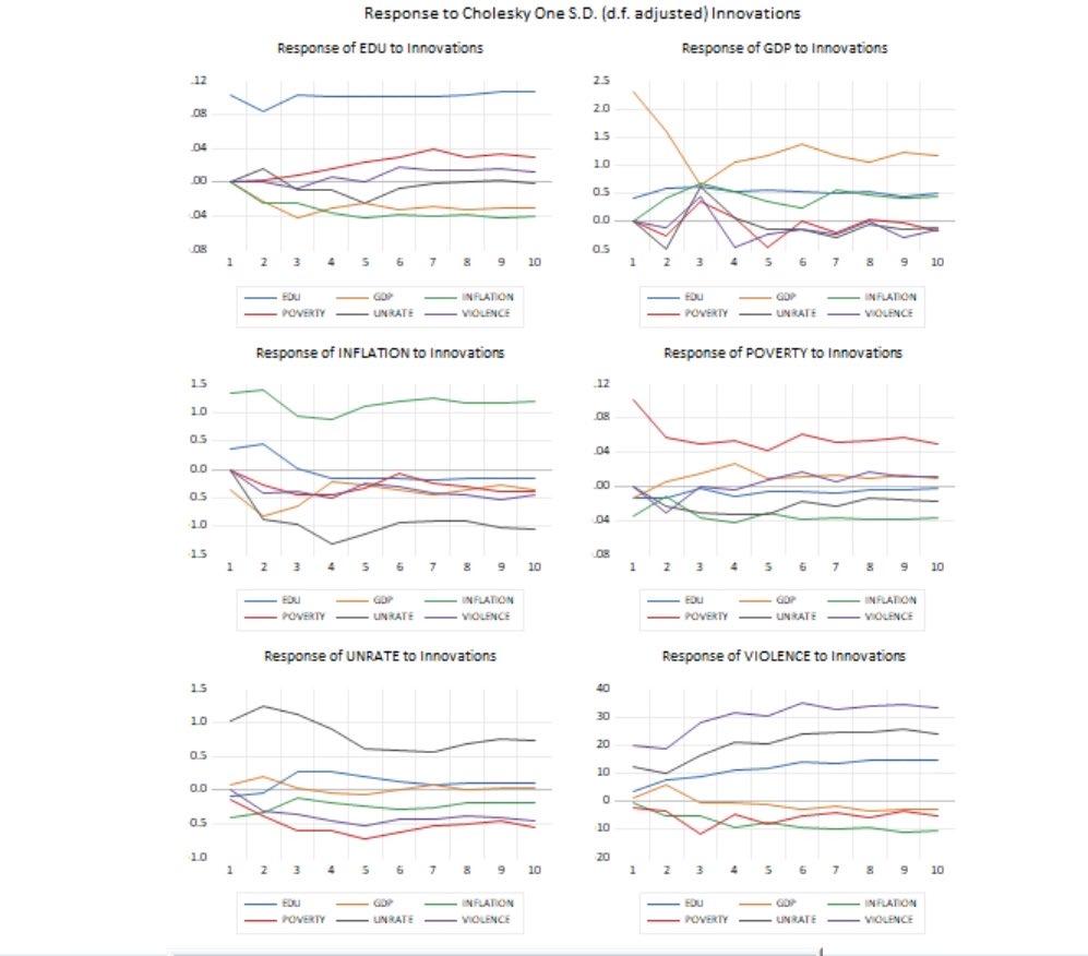
298
The impulse response functions as shown in table 4 show the effect on each independent variable on domestic violence. This is the response to Cholesky one standard deviation adjusted by the independent variable, and how the response controls itself overtime. As you can see, the impact of an increase in education on domestic violence is Negative. The more education one has, the less domestic violence. An increase in the unemployment rate and domestic violence is shown to be positive. As more unemployment creates more stress, and more blame on the other partner. It also leaves more time for domestic abuse to occur. The effect of one standard deviation on poverty as well as inflation is also positive, as for the same reasons along with unemployment. Stress about money creates more violent tendencies, as well as those who are in areas with high poverty in the United States probably have less access to resources, less education on domestic violence, and less police protection.
5.1 POLICY IMPLICATIONS
Inflation and unemployment were statistically significant in showing that there is enough data to prove these variables are correlated to domestic violence in the long term, but do not directly cause one another. Economic instability can lead to crime, with the association of other factors that may cause domestic violence, i.e., mental health, alcoholism, or drug abuse from poor economic outcomes. If the FED creates better monetary policy decisions as well as utilize more monetary policy tools like quantitative easing or tightening, and raising the federal funds rate, it can affect the amount of inflation and unemployment overall. Policy makers can also work to provide better job placement programs for those who are in poverty, provide continual government support such as SNAP benefits, low-income housing, better education for children in povertystricken areas, this can all contribute to change in the rates of domestic violence when just considering the independent variables within this study.
5.2 LIMITATIONS OF STUDY
Limitations of the study include this analysis only being run with country specific data over many years. If I had used state specific data, I might have been able to identify a difference among states, in various regions, and how inflation and unemployment, which makes up the misery index, might have more of an effect on domestic violence more than
299
other states. I also believe that some areas may be more prone to higher domestic violence rates due to other factors, and overall crime rates being high in specific states. If factors such as poverty are more prevalent in some areas, it could already be a basis for more domestic violence. I also think that state specific analysis could be broken into doing an urban vs rural analysis to see if in major cities domestic violence is higher because of the effect of the misery index. Lastly, within my research I ran my Granger causality test with the Misery index data as two separate variables, inflation, and unemployment. If I ran these variables together and added other variables into the model, it could change the overall causality results.
5.3 CONCLUSION
This study showed that in the long run, there is no causality between violence and the independent variables, at least in the United States. Using time series annual data, Granger causality tests were conducted, after an ADF and Unit Root test were done. The objective was to determine whether the Misery Index caused an increase in domestic violence, which it did not. In summary, based on the results, the study goes against the hypothesis based on prior literature for other countries, especially Saburo et. al (2017), that stated in democratic regimes, people are three times more likely to be miserable, from inflation and unemployment, than countries in a dictatorship. In the United States this was not true as a nation overall. This may be because of current monetary policy and other fiscal policy that helps citizens, compared to countries such as Pakistan, which although may be democratic, may not have the same social and economic standards as the United States, which lowers the rate of domestic violence.
300
Appendix A: Variable Description and Data Source
Acronym Description
MI Misery Index calculated from annual unemployment and inflation
LDGP The logarithm of GDP per capita, PPP (current international $)
POV Percent of 100,000 under $5.50 USD wage
I Inflation – Consumer Prices (annual %)
UN
Unemployment Rate total (% of the total labor force)
Crimel Rate of domestic violence per 100,000
Data source
FRED
FRED
World Bank
FRED
FRED
EDU
Average rate of education
US Department of Justice
Human Development Index
301
REFERENCES
Ajide, F. M. (n.d.). Institutional Quality, Economic Misery and Crime Rate in Nigeria. Sciendo. Retrieved April 25, 2023, from https://sciendo.com/es/article/10.2478/eb-2019-0012
Criminal Victimization, 2021 | Bureau of Justice Statistics. (2022, September 20). Bureau of Justice Statistics. Retrieved April 25, 2023, from https://bjs.ojp.gov/library/publications/criminalvictimization-2021
Inflation, consumer prices for the United States (FPCPITOTLZGUSA) | FRED | St. Louis Fed. (n.d.). FRED. Retrieved April 25, 2023, from https://fred.stlouisfed.org/series/FPCPITOTLZGUSA National Statistics. (n.d.). National Coalition Against Domestic Violence. Retrieved April 25, 2023, from https://ncadv.org/STATISTICS
Piraee, K., & Barzegar, M. (2022, July 29). The Relationship between the Misery Index and Crimes: Evidence from Iran. journal Asian Journal of Law and Economics. Retrieved April 25, 2023, from https://www.degruyter.com/document/doi/10.2202/2154-4611.1018/pdf
Reyhan Cafrı Açcı, & Pınar Çuhadar. (n.d.). Unemployment or Inflation? What Does the Misery Index Say about the Causes of Crime?*. Open METU. Retrieved April 25, 2023, from https://open.metu.edu.tr/bitstream/handle/11511/96796/1136-7319-2-PB.pdf
Saboor, A., Sadiq, S., & Hameed, G. (2016, May 02). Dynamic Reflections of Crimes, Quasi Democracy and Misery Index in Pakistan. Social Indicators Research volume. Retrieved April 25, 2023, from https://link.springer.com/article/10.1007/s11205-016-1348-8
Tang, C. F., & Lean, H. H. (2009, 02). New evidence from the misery index in the crime function Economic Letters. Retrieved April 25, 2023, from https://www.sciencedirect.com/science/article/abs/pii/S0165176508003200
Unemployment Rate+Consumer Price Index for All Urban Consumers: All Items in U.S. City Average | FRED | St. Louis Fed. (n.d.). FRED. Retrieved April 25, 2023, from https://fred.stlouisfed.org/graph/?g=IenV
Unemployment Rate (UNRATE) | FRED | St. Louis Fed. (n.d.). FRED. Retrieved April 25, 2023, from https://fred.stlouisfed.org/series/UNRATE
302
How International Trade and Government Integrity Affect
the Structural Transformation of Lao PDR and Cambodia
Yixin Wan
Abstract:
This paper explores the how international trade and government integrity affect the structural transformation of Lao PDR and Cambodia. This empirical study is conducted by using the methodology based on Chenery-Syrquin model with several control groups that have impacted on structural transformation in Lao PDR and Cambodia. Moreover, the obtained data is from 1993 to 2021 to find out how these two countries transform from being agriculture dominant economy to being more industry-and services-oriented economy. This study has confirmed non-linear effects of both income and population on the sectoral shares and found that trade has facilitated structural transformation in Lao PDR but that didn’t happen in Cambodia. The political corruption index affected the sectional sectors in different ways in Lao PDR and Cambodia, but the results are not statistically significant.
JEL Classification: F14, F62, F63, F43, H11
Keywords: Trade, Role of Government, Economic Development, Economic impacts of globalization
303
1.0 INTRODUCTION
The transformation of economics is long running interest topic for scientists focused on the development economics. As the previous study (Hnatkovska and Lahiri, 2014), the structural transformation of economics is closely related to the process of development. The process of structural transformation is characterized by systematic changes in the reallocation of economic productive factors, which shift from the primarily agricultural activities to the industrial and service sectors (Restuccia,2011). By shifting the productive factors towards to export, international trade is a force in expediting the structural transformation (Federico and TenaJanguito, 2019). Additionally, the governance and political system play an important role in long-term economic growth. The governance performance, such as corruption and lack of regulation, would bring uncertainty into economic relationships and lead to economic inefficiency (Derviş, 2016).
There are many similarities between Lao PDR and Cambodia. For example, there are some similar characteristics of the political socio-cultures for these two countries. The similar political structure, described by Oliver Wolters as Mandala, is as circles of power forming part more encompassing circles of power. According to Boike Rehbein (2005), Mandala still has a deep influence in the political structure in these areas. For both countries, patrimonial is the primary characteristic of the political culture. However, there are also differences between two countries. Compared to Lao PDR, Cambodia has a bigger population, which means the larger number of labors and higher population density. Additionally, Cambodia is less mountainous with the access to ocean, whereas Lao PDR has none. Within this ambient, this paper is going to explore the relationship among trade openness, structural change and government integrity for Lao PDR and Cambodia.
This paper is structured as follows: Section 2 gives the brief trend and stylized facts. Section 3 gives the brief literature review. Section 4 gives data sources and an extensive discussion for the empirical methodology based on Chenery-Syrquin model. The panel diagnostic tests and estimation results are in Section 5 while the Section 6 concludes the paper with economic and political thoughts.
2.0 TREND AND SYLIZED FACTS
304
This section outlines some stylized facts on the structural transformation of Lao PDR and Cambodia, which includes the changing structure of production, and to what extent the economic composition of these two countries has shifted towards the industrial and service sectors over time.
In general, Figure 1 illustrates that the share of agriculture has declined over time for both countries. For Cambodia, the share of agriculture experienced a slightly increase from 1993 to 1995 then generally declined with some fluctuations. It continued to decline until 2019 reaching the lowest point of 20.712%. From 2019 to 2021, the share of agriculture increased slightly, but still remained below 25%. For Lao PDR, the share of agriculture experienced a gradually decrease from 1990 to 1995 then increased again with a peak of 51.853% in 1997. It continued to decline until 2018 reaching the lowest point of 15.709%. From 2019 to 2021, the share of agriculture increased slightly, but still remained below 17%. Overall, the share of agriculture in Lao PDR and Cambodia has been declining since the early 1990s, with some fluctuations along the way. Additionally, the share of agriculture for both countries experienced a slightly increase after 2019.
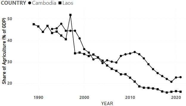
Source: Author’s calculation; data collected from World Development Indicators, World Bank.
Figure 2 shows a general increasing trend in the share of industry in both countries from 1993 to 2021 with some fluctuations. For Cambodia, the share of industry only accounted for 12.646% of the economy in 1993, which had risen to 36.835% by 2021. However, it's also noted that there is a slight decrease in 2007 which is followed by a sharp drop in 2008 and 2009. For
Figure1: Share of agriculture as percentage of GDP
305
Lao PDR, there is a general increasing trend over the past few decades. The share of industry increased to a peak of 32.437% in 2012, but there is sharp drop to from 2012 to 2014 then recovered to 34.130% in 2021.
Figure2: Share of industry as percentage of GDP
Figure 3 shows both countries have experienced significant changes in the share of services in their economies over the past few decades, with an upward trend in Cambodia before 2019 and fluctuating trend for Lao PDR.
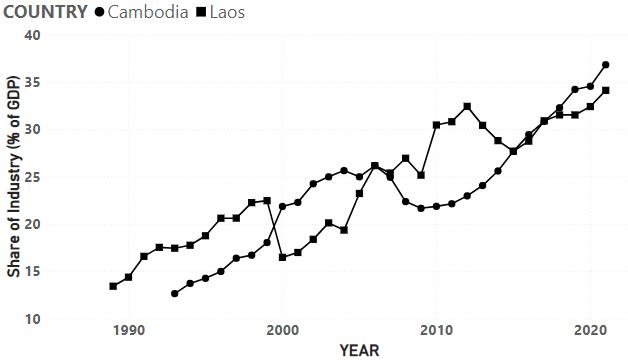
For Cambodia, the total trend for share of services was increasing from 1993 to 2019 but experienced a slight decline from 2007 to 2008 and a sharp decline in 2020 and 2021. It increased from 7.3% in 1993 to a 34.0% in 2012, then keep stable around 34% until 2019. However, it dropped sharply to 14.7% in 2020, and keep decreasing to 10.2% in 2021. For Lao PDR, it shows a fluctuating trend in the share of services in the past decades. There is a clear upward trend from before 1998 but dropped sharply in 1999 and remained relatively stable at a lower level until 2008. From 2008 to 2019, it shows a gradual increase trend with some fluctuations, but dropped sharply again in 2020 and 2021.
Figure3: Share of services as percentage of GDP
Source: Author’s calculation; data collected from World Development Indicators, World Bank.
306
Source: Author’s calculation; data collected from World Development Indicators, World Bank.
3.0 LITERATURE REVIEW
Traditional explanations of the structural transformation based on one or both of two mechanisms (Chenery and Srinivasan, 1988): (i) the income elasticity of demand for agriculture products is less than one and (ii) faster total factor productivity growth in agriculture sector relative to other sectors in the economy. The first mechanism implies that as the economy grows, the demand for farm goods decreased, consequently, the labor working for agriculture declines. The second mechanism implies that fewer labor force is needed to produce the same amount of farm goods.
Duarte and Restuccia (2010) investigated the structural transformation through reallocation of labor across countries, which implied the first mechanism: the demand for farm goods would decrease as the economy grows up. For countries featuring low productivity in all sectors, they found that a big share of labor was allocated to agriculture while a small share of labor was allocated to services and industries. With positive productivity growth in all sectors, labor would be reallocated away from agriculture toward industry and services. According to another research published in 2006, Duarte and Restuccia found the structural transformation helped the GDP growth in Portugal from 1956 to 1995. During this period, a bigger share of labor was allocated to industry, and in turn, the smaller share of labor was allocated to agriculture and services sectors.
Caselli and Coleman investigated the U.S. Structural Transformation and Regional Convergence, which implied the second mechanism: structural transformation is caused by a faster productivity growth in agriculture sector. Due to the declining education/training costs, an
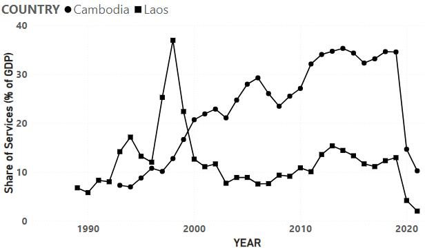
307
increasing proportion of the labor force is shifting away from the (unskilled) agriculture sector and toward the (skilled) non-agricultural sector.
According to United Nations Department of Economic and Social Affairs in 2017, international trade always played a role in supporting the economic growth and poverty alleviation in many nations. In some countries, the economy relied on export-led growth to accelerate structural transformations toward industrial and services factors. Spatafora et al. also mentioned the importance of international trade in stimulating the development of the service sector as percentage of GDP. In 2007, the cross-border service exports have been recorded amounted to $3.3 trillion, as 20% of the total trade globally.
Generally, the empirical research focusing on the effectiveness of international trade on structural transformation are based on two frameworks: (i) non-homothetic preferences, and (ii) asymmetric sectoral productivity growth. The first framework, non-homothetic preferences, is a demand-side mechanism emphasized that the consumption basket would shift towards to manufactured goods from the agricultural products as the countries become richer. The second framework, Baumol effect (also called asymmetric sectoral productivity growth), is a supply-side mechanism emphasized that the share of agriculture, industry, and services would change overtime.
Through the demand-side mechanism, Erten and Leight (2021) studied how exports surge in China led to the structural changes after joining the WTO. As the uncertainty of tariff had decreased, the surge in manufactured product exports boost the economic growth which led to a structural transformation.
Through the supply-side mechanism, McCaig and Pavcnik (2018) studied the reallocation of productive factors between informal and formal enterprises under the manufacturing sector in Vietnam after the 2001 US-Vietnam Bilateral Trade Agreement. They found that the proportion of labor working in informal household enterprises decreased significantly compared to formal enterprises. As productivity increased due to international trade, McCaig and Pavcnik documented how the productive factors were re-allocated within industry sector in Vietnam.
Although there is no direct evidence showing how government performance and integrity affect the structural transformation, it is widely recognized that they have significant effects on the economic development. According to J. Liu et al. in 2018, good governance performance
308
would bring a significant positive effect on developing the economy. Additionally, good governance is also regarded as playing a role in reducing risk for investors and attracting foreign direct investment. Mengistu and Adhikary (2011) investigates how governance affect the foreign direct investment (FDI) inflows in 15 Asian countries from 1996 to 2007. They found that six components of good governance, including control of corruption, are the key determinants of FDI inflows.
4.0 DATA AND EMPIRICAL METHODOLOGY
4.1 Data
Time series data on most of the economic factors, GDP per capita (current $US), and share of agriculture, industry and services as percentage of GDP, is from the World Development Indicators (WDI) 2022. The population data is from U.S. Census Bureau. Data on Foreign direct investment inflows ($US millions) are sourced from UN Conference on Trade and Development. Data on government integrity is expressed as political corruption index (0-1, higher is more corrupt) using a model estimated method from V-Dem Institute. The data period for Cambodia is from 1992 to 2021 and for Lao PDR is it is from 1989 to 2021. The summary statistics of each country is given in the following Table 1 and Table 2. The Table 1 reveals highest volatility in share of services and lowest volatility in share of industry in Cambodia. The Table 2 reveals highest volatility in share of agriculture and lowest volatility in share of industry in Lao PDR
Variable N Mean Std. dev. Min Max Share of agriculture 29 33.023 7.885 20.712 47.725 Share of industry 29 23.741 6.360 12.646 36.835 Share of services 29 23.236 9.613 6.953 35.291 Ln (GDP per capita) 29 6.418 0.663 5.511 7.421 Ln (GDP per capita) ^2 29 41.612 8.571 30.369 55.077 Ln (POPULATION) 29 16.428 0.123 16.188 16.621 Ln (POPULATION) ^2 29 269.908 4.046 262.037 276.245 Ln (FDI inflows) 29 6.382 1.375 3.991 8.206 Polit. corruption index 29 0.894 0.011 0.863 0.899
Table 1. Summary Statistics of Variables for Cambodia
309
Table 2. Summary Statistics of Variables for Lao PDR
4.2 Empirical Model
The model for this study is adopted from the principal specification of Chenery and Syrquin (1975) and Syrquin and Chenery (1989) for structural transformation:
ln ������������ = ����0 + ����1(ln������������) + ����3(ln������������) + ������������, (1) where, the variable ������������ represents the shares of different sectors, namely agriculture, industry, and services as percentage of GDP of country ���� at time ���� ������������ denotes the per capita GDP of country ���� at time ����, which reflects the income level. ������������ represents the population of country ���� at time ����. The equation (1) aims to demonstrate that output share of each sector is influenced by both per capita income and size of the population.
Chenery and Taylor (1968) introduced a quadratic term in their model as it was evident that diminishing income elasticities would be observed with increasing income levels. Later, Chenery and Syrquin (1989) adopted a more general specification to capture the non-linear effects of both income and population. That specification is presented below:
������������ = ����0 + ����1(ln������������) + ����2(ln������������)2 + ����3(ln������������) + ����4(ln������������)2 + ������������, (2)
In order to determine how international trade and government integrity affect the structure transformation, variable capturing FDI inflows and political corruption index are added into Equation (3):
Variable N Mean Std. dev. Min Max Share of agriculture 33 29.678 11.436 15.709 51.853 Share of industry 33 23.941 6.187 13.428 34.130 Share of services 33 12.009 6.416 2.004 36.948 Ln (GDP per capita) 33 6.507 0.933 5.137 7.863 Ln (GDP per capita) ^2 33 43.181 12.391 26.393 61.822 Ln (POPULATION) 33 15.572 0.183 15.225 15.850 Ln (POPULATION)^2 33 242.505 5.691 231.798 251.211 Ln (FDI inflows) 33 4.712 1.871 1.386 7.430 Polit. corruption index 33 0.763 0.008 0.733 0.770
������������ = ����0 + ����1 (ln������������) + ����2(ln������������) ² + ����3 (ln������������) + ����4(ln������������) ² + ����5(ln FDI����) + ����6(Government Integrity����) + ������������, (3) 310
5.0 EMPIRICAL RESULTS
The regression results are given in Table 3 and Table 4.
Table 3. Regression Results for Cambodia
The results showed in Table 3 pointed some interesting insights on the factors affecting structural transformation in Cambodia.
Considering the positive relationship between share of agriculture and GDP per capita, as the share of agriculture in a country's economy increases, GDP per capita tends to increase but at a decreasing rate. Since share of agriculture is negatively related to GDP per capita square, the growth in the share of agriculture tends to slow down as the GDP per capita increases. Conversely, as the share of industry in a country's economy increases, GDP per capita tends to decrease but the decreasing trend would slow down as GDP per capita further increases. The table also suggests that the relationship between the share of agriculture/industry/services and GDP per capita is not linear but characterized by a non-linear U-shaped relationship. For share of services, it is both positively related to GDP per capita and GDP per capita square, which means
Share of Agriculture Share of Industry Share of Services Ln (GDP per capita) 21.51 (0.46) -15.93 (-0.49)* 212.3* (-2.49) Ln (GDP per capita) ^2 -1.924 (-0.47) 0.706 (0.25) 20.56** (2.82) Ln (POPULATION) -1253.7 (-0.34) -3216.4 (-1.26) 33437.6*** (5.04) Ln (POPULATION)^2 35.33 (0.31) 101.4 (1.29) -1023.6*** (-5.04) Ln (FDI inflows) 5.077*** (3.82) -2.708** (-2.94) -5.213* (-2.18) Polit. corruption index 24.86 (0.54) 10.17 (0.32) -74.85 (-0.91) Constant 10980.8 (0.37) 25587.3 (1.23) -272409.8*** (-5.06) Observations 29 29 29 Adjusted R-squared 0.919 0.940 0.822 F-statistic 53.62 73.82 22.58 Prob. F-statistic 0.0000 0.0000 0.0000 RMSE 2.2506 1.5608 4.0532 Note: t statistics in parentheses, * p<0.05, ** p<0.01, *** p<0.001
311
the positive relationship between the share of services and GDP per capita would strengthen as GDP per capita increases.
While the share of agriculture and industry are negative related to Population but positive related to the Population square. That means the share of agriculture and industry in Cambodia tends to decrease as the population of a country increases, in other words, the economic growth may be associated with a larger share of agriculture/industry with a low level of population while the it may be associated with a larger share of services with higher level of population. For share of services, it is positively related to Population but negatively related to Population square, which means the share of services in Cambodia tends to increase as the population of a country increases. Due to negative coefficient on the Population square term, the relationship between the share of services and population is not linear but an inverted U-shaped relationship, which means the positive relationship would weaken as the population increases beyond a certain threshold. It indicates that there may be increased competition for resources and labor with a very high level of population, which makes the service sector fail to continue to grow at the same rate.
As far as the role of trade is concerned, it notes that the FDI inflows has statistically significant effect on shares of agriculture, industry, and services. While trade has positive impact on agricultural share, it has negative impact on industrial and services sector in Cambodia. This means that trade tends to benefit the agricultural sector more than industrial and services sectors. Despite the impact of FDI inflows, the agricultural sector remains an important part of Cambodia's economy. Hence, it infers that the overall agricultural orientation is still existing in Cambodia.
Concerning the role of political corruption, it notes that the political corruption index is positive related to the share of agriculture/industry while it is negative related to the share of services. It means that as the level of political corruption in Cambodia increases, the share of services would decrease while the share of agriculture/industry would increase. Since the significance level of political corruption index coefficients are not starred, they aren’t statistically significant.
To promote the growth of the service sector in Cambodia, government could accomplish that through providing necessary infrastructure, financial incentives, and implement anticorruption measures to reduce the level of political corruption. As agricultural orientation is still
312
existing in Cambodia, the government could implement policies to promote sustainable agriculture practices, such as investing in agricultural technologies to increase productivity and encouraging the use of renewable energy sources in agricultural activities.
The negative relationship between the share of agriculture/services and GDP per capita indicates that as the GDP per capita increases, the share of agriculture/services in the economy tends to decrease but the decreasing trend would slow down as GDP per capita further increases due to the positive relationship with GDP per capita squared. On the other hand, the positive relationship between share of industry and GDP per capita means that the share of industry tends to increase as GDP per capita increases, but the increasing trend would slow down as GDP per capita further increases due to the negative relationship with GDP per capita squared. This table
Share of Agriculture Share of Industry Share of Services Ln (GDP per capita) -39.77 (-1.14) 29.12 (1.25) -231.5*** (-5.20) Ln (GDP per capita) ^2 3.528 (1.17) -2.240 (-1.12) 18.01*** (4.69) Ln (POPULATION) 4464.7 (1.43) -1622.3 (-0.78) 12933.1** (3.26) Ln (POPULATION)^2 -146.6 (-1.45) 52.89 (0.79) -417.8** (-3.25) Ln (FDI inflows) 0.114 (0.11) 1.214 (1.84) 2.978* (2.35) Polit. corruption index -286.0* (-2.08) 16.85 (0.18) -65.72 (-0.38) Constant -33613.2 (-1.41) 12348.7 (0.78) -99298.1** (-3.27) Observations 33 33 33 Adjusted R-squared 0.931 0.896 0.644 F-statistic 72.61 46.77 10.66 Prob. F-statistic 0.0000 0.0000 0.0000 RMSE 3.0106 1.9985 3.8271 Note: t statistics in parentheses, * p<0.05, ** p<0.01, *** p<0.001
Table 4. Regression Results for Lao PDR
Table 4 also presents some intriguing findings on the factors affecting structural transformation in Lao PDR
313
also suggests a U-shaped relationship between the share of agriculture/industry/services and GDP per capita in Lao PDR.
The share of industry is negative related to Population but positive related to the Population Square. That means the share of industry in Lao PDR tends to decrease as the population increases, in other words, the economic growth may be associated with a larger share of industry with a low level of population while the it may be associated with a larger share of agriculture/services with higher level of population. For share of agriculture/services in Lao PDR, it is positively related to Population but negatively related to Population Square, which means the share of agriculture/services in Cambodia tend to increase as the population of a country increases but the positive relationship would weaken as the population increases beyond a certain threshold.
As far as the role of trade is concerned, it notes that the FDI inflows only has significant effect on shares of industry and services since the share of agriculture increase 0.11% as FDI inflows increase 1%. Compared to agriculture, FDI has a greater impact on industry and services while it benefits the services sector more than industry sector. Despite the impact of FDI inflows, it infers that an industry/services orientation has been happening in Lao PDR.
Concerning the role of political corruption, it notes that the political corruption index is positive related to the share of industry while it is negative related to the share of agriculture/services. It means that as the level of political corruption in Cambodia increases, the share of agriculture/services would decrease while the share of industry would increase.
Since Lao PDR are benefiting from foreign investment in increasing the share of industry/services, the government could keep attracting FDI by creating a more business-friendly environment, providing tax breaks, and offering financial incentives to attract the foreign investors. It also indicates that the government corruption is hindering the growth of the agriculture and services sectors. Hence, the government could increase transparency and strengthen legal frameworks to tackle this issue.
The study assumes that the relationship between all dependent and independent variables is homogeneous across all regions in Cambodia and Lao PDR. For some variables, they are not statistically significant. Additionally, the tables didn’t account for potential interactions or nonlinear relationships between the variables. There may also be multicollinearity issues between the independent variables, which can affect the reliability of the coefficients and p-values.
314
5.0 CONCLUSION
The structural transformation is a key characteristic of economic development. The primary aim of this paper is to examine if trade and government integrity plays a role in the process structural transformation in Lao PDR and Cambodia.
Data suggests that the share of agriculture of both countries has experienced a decline with some fluctuations along the way from 1990s to 2021. For the share of industry, it showed an increasing trend with some fluctuations in both countries, but there is a sharp drop from 2008 to 2009 in Cambodia and from 2012 to 2014 in Lao PDR. For the share of services, there is an increasing trend for Cambodia and a fluctuating trend for Lao PDR.
In order to assess to role of trade and government integrity in structural transformation of Lao PDR and Cambodia, this paper used the Chenery-Syrquin model to estimate how different factors affect the structural transformation. In summary, the main findings are as follows: First, this study confirmed non-linear effects of both income and population on the sectoral shares. Secondly, the results support that trade has facilitated structural transformation in Lao PDR but that didn’t happen in Cambodia. Remaining protective of the agriculture sectors could be a reason to explain the phenomenon happened in Cambodia. Thirdly, the political corruption index is only negatively related to share of services in Cambodia and only negatively related to share of agriculture/services in Lao PDR. Additionally, the coefficients for the political corruption index are not statistically significant.
315
Reference list:
Viktoria Hnatkovska and Amartya Lahiri. “The Rural-Urban Divide in India.” IGC, Jan. 2012.
Derviş, Kemal. “Good Governance and Economic Performance.” Brookings, 28 Sept. 2016, www.brookings.edu/opinions/good-governance-and-economic-performance.
Giovanni Federico and Antonio Tena Junguito. Federico-Tena World Trade Historical Database: World Trade. 24 Jan. 2018, https://doi.org/10.21950/jkzfdp.
Restuccia, Diego. Recent Developments in Economic Growth. 1 Sept. 2011, papers.ssrn.com/sol3/papers.cfm?abstract_id=2190597.
United Nations [Department of Economic and Social Affairs]. Global Context for Achieving the 2030 Agenda for Sustainable Development: International Trade: Development Issues No. 7. Feb. 2017, www.un.org/development/desa/dpad/publication/development-issues-no-7global-context-for-achieving-the-2030-agenda-for-sustainable-developmentinternational-trade.
Spatafora, Anand, Mishra. “Structural Transformation and the Sophistication of Production.”
IMF Working Paper, vol. 12, no. 59, International Monetary Fund, Feb. 2012, p. 1. https://doi.org/10.5089/9781463937775.001.
Bilge Erten and Jessica Leight. “Exporting Out of Agriculture: The Impact of WTO Accession on Structural Transformation in China.” The Review of Economics and Statistics, vol.103, no. 2, The MIT Press, May 2021, pp. 364–80. https://doi.org/10.1162/rest_a_00852.
Brian McCaig and Nina Pavcnik. “Export Markets and Labor Allocation in a Low-Income Country.” The American Economic Review, vol. 108, no. 7, American Economic Association, July 2018, pp. 1899–941. https://doi.org/10.1257/aer.20141096.
Liu, Tang, Zhou, Liang. “The Effect of Governance Quality on Economic Growth: Based on China’s Provincial Panel Data.” Economies, vol. 6, no. 4, MDPI, Oct. 2018, p. 56.
https://doi.org/10.3390/economies6040056.
Alemu Mengistu and Bishnu Kumar Adhikary. “Does Good Governance Matter for FDI Inflows? Evidence From Asian Economies.” Asia Pacific Business Review, vol. 17, no. 3, Taylor and Francis, July 2011, pp. 281–99. https://doi.org/10.1080/13602381003755765.
316
Exploring the Relationship Between Exchange Rate Pass-Through and CPI Inflation in Mainland China
and India
Edward Zhou
Abstract:
By examining the link between exchange rate transmission and cpi inflation across countries, we investigate whether there is a considerable link between the two. In this paper, we examine data for two representative Asian countries, mainland China and India, to determine whether there is a relationship between the two. The study finds no significant link between exchange rate and cpi inflation for China by comparing 40 years of data for these two countries, but for India, there is a particularly clear link. The difference between the two is mainly due to the different exchange rate control systems implemented by the two governments. The paper will explore and test this further to find if there is a link between the two and which factor has the greatest impact on the exchange rate.
JEL Classification: E40,E44,E47
Key words: ERPT(exchange pass through rate), CPI, PPI,IMP,NEER
Edward zhou is an accounting student study in Bryant university, he can be reach at: 1150 Douglas pike, Smithfield, RI02917, USA. Email: dzhou1@bryant.edu; phone: +(401)556-4870.
317
The dynamics of exchange rates and inflation have been a very important point of debate in economics, especially in macroeconomics. There are many exchange rate regimes in place around the world, such as the fixed exchange rate in China, the flexible exchange rate regime in the United States and the euro-using region, and the managed floating exchange rate regime in India, which tend to influence these dynamics (Mallick and Marques, 2008). Whereas China has been in a state of massive inflation since the second half of 2007, India has seen inflation enter an inflationary era since 2010.
This study aims to enhance understanding exchange rate pass-through (ERPT) is a term used to describe the degree to which changes in exchange rates affect domestic inflation in an economy. It refers to the extent to which changes in the exchange rate of a country's currency are transmitted to the prices of goods and services produced within that country. The relationship between exchange rates and interest rates can also be influenced by the position of an economy, which can further impact ERPT. Various definitions of ERPT are available in the literature: “Exchange rate pass-through is the percentage change in the local currency importing countries.” – (Goldberg and Knetter 1997).
In recent years, as inflation has grown and spread around the world, a large number of governments have initiated attempts to control the exchange rate in the hope of controlling the rate of inflation, but none of the results have been significant. This paper will explore whether there is a specific link between exchange rate pass through and CPI inflation.
The rest of the paper is organized as follows: firstly, this paper will look for the inflation in mainland China and India in recent years. Secondly it will explore the exchange rate changes and trends in these two countries. Thirdly, this paper will measure whether there is a stable and persistent link between the two through the range causality. Section two of the paper provides a summary of the existing literature on the topic. Section three presents the theoretical framework, data sources, and regression analysis used in the study. The empirical methodology employed in the analysis is explained in section four. Section five offers a detailed discussion of the empirical findings, while section six provides policy implications and draws conclusions based on the study's results.
1.Introduction:
318
2.0 Trend:
Figure 1 and 2 shows the development of inflation in India with the development of the economy. It can be found that the overall trend of inflation rate in India is getting faster and faster, and a big problem is that the magnitude of change is very large, every year, sometimes positive, sometimes negative, which indirectly reflects the situation of the domestic economic situation is very free. Comparing the exchange pass through rate of India, we can see that the currency has been devalued by up to double from one dollar to 43 Indian currency in 2005 to one dollar to 82 Indian currency now. And that's with the exchange rate converting in the face of general global inflation. That means that with the dollar already depreciating, the Indian currency is still depreciating at up to double the rate. This would be a particular exaggeration. This is something that will be explored later in this article, whether the exchange pass through rate is changing back and forth because of the change in cpi inflation.
Figure 1: The exchange rate pass through in India
Source: world bank database
0.000 10.000 20.000 30.000 40.000 50.000 60.000 70.000 80.000 1982 1984 1986 1988 1990 1992 1994 1996 1998 2000 2002 2004 2006 2008 2010 2012 2014 2016 2018 2020
Figure 2: The import price and producer price index in India
319
Exchange rate pass through(India)
Figure 3 turning back to China, another one of the two largest Asian economies, as the economy continues to grow after the reform and opening up, with the total quickly jumping to the top of the world, the first thing we will observe is the change in the inflation rate in China. China's inflation rate also varies considerably, but in terms of total magnitude, it is slightly lower than India's and has smaller positive and negative maximum and minimum values than India's maximum and minimum values. China's inflation outbursts were mainly concentrated before 2010, and inflation rates have been relatively low and stable in recent years.
Exchange rate pass through(China)
Source: world bank database
Figure 3: The exchange rate pass through in Chin
-10.0% 0.0% 10.0% 20.0% 30.0% 40.0% 50.0% 60.0% 0 1E+11 2E+11 3E+11 4E+11 5E+11 6E+11 7E+11 1982 1985 1988 1991 1994 1997 2000 2003 2006 2009 2012 2015 2018 2021 INDIA Import price PPI 0 1 2 3 4 5 6 7 8 9 10 1982 1984 1986 1988 1990 1992 1994 1996 1998 2000 2002 2004 2006 2008 2010 2012 2014 2016 2018 2020
Source: world bank database
320
Figure 4 observing the change in the exchange pass through rate back in China, there is not a particularly significant change from 8.2 RMB per dollar in 2005 to 6.8 RMB per dollar now, which is not a particularly significant change and relatively speaking the RMB has appreciated. This is a particularly stark contrast to the doubling of India's situation, which is an indirect indication that economic development does not have to depend on exchange rate devaluation to proceed faster. Of course, this paper will also look at the reasons why this is happening, whether it is a result of the relative stability of the nation's own money circulation and the rise of the country's economic power in the world, or whether it is simply a result of the government's constant control to force the currency from depreciating too quickly, which is also a result of the difference in the two countries' political systems.
3.0 Literature review:
Exchange rate pass-through (ERPT) is an important issue in international economics as it determines how changes in exchange rates affect domestic prices and ultimately, inflation. Various studies have been conducted to examine the extent and determinants of ERPT across different countries and regions.
Mihaljek and Klau (2001) estimated the extent of ERPT for thirteen emerging market economies using the single equation method. However, they ignored possible regime changes in
Figure 4: The import price and producer price index in China
Source: world bank database
-10.0% -5.0% 0.0% 5.0% 10.0% 15.0% 20.0% 25.0% 0 5E+11 1E+12 1.5E+12 2E+12 2.5E+12 3E+12 1982 1984 1986 1988 1990 1992 1994 1996 1998 2000 2002 2004 2006 2008 2010 2012 2014 2016 2018 2020 CHINA Exchange rate pass through Import price CPI PPI 321
exchange rate policies. In contrast, McCarthy (2000), Hahn (2003), and Faruqee (2006) used the VAR approach to examine ERPT in developed countries, particularly in the Euro Area. Ito and Sato (2006) applied the VAR analysis to ERPT in East Asian countries, while Belaish (2003) and Leigh and Rossi (2002) used the VAR technique for Brazil and Turkey, respectively.
In addition to the methodological differences in examining ERPT, researchers have also explored the factors that affect ERPT. Dornbusch (1987) proposed the overshooting hypothesis, which suggests that ERPT is higher in the short run as prices adjust slowly to changes in exchange rates. Engel and Storgaard (2004) argued that ERPT is influenced by the degree of competition in domestic markets and the pricing strategies of firms. Marazzi and Rothenberg (2006) found that ERPT is higher when exchange rate volatility is higher. Bhattacharya et al. (2008) suggested that ERPT is affected by the degree of openness of the economy, the structure of trade, and the monetary policy regime.
Belaisch (2003) explores the issue of ERPT in Brazil, using a VAR model. The study finds evidence of significant pass-through from exchange rates to domestic prices, although the extent of pass-through varies depending on the type of shock and the time horizon considered. The study also highlights the role of inflation expectations and the degree of market competition in influencing the magnitude of pass-through.Burstein et al. (2002) and (2005) investigate the puzzle of why inflation rates remain low after large devaluations in several emerging market economies. Using a dynamic general equilibrium model, the authors find that the presence of nominal rigidities in pricing and wage-setting behavior can explain the observed phenomenon. The study highlights the importance of considering the underlying economic structure when assessing the effects of exchange rate changes on domestic prices.Campa and Goldberg (2005) examine ERPT into import prices in a cross-section of countries. Using panel data techniques, the authors find evidence of incomplete pass-through, with the extent of pass-through varying across countries and over time. The study also highlights the role of pricing-to-market behavior and competition in influencing the magnitude of pass-through.Campa et al. (2005) focus specifically on the euro area, using a similar approach to investigate ERPT into import prices. The study finds evidence of incomplete pass-through, with the degree of pass-through varying across product categories and across countries within the euro area. The study also highlights the role of exchange rate volatility in influencing the magnitude of pass-through.
322
Overall, the literature suggests that ERPT varies across countries and regions, and is influenced by various factors such as exchange rate volatility, market competition, trade openness, and monetary policy regimes. Further research is needed to better understand the determinants of ERPT and its implications for macroeconomic stability.
4.0 Data, Variables and Empirical Methodology
4.1. Data and Variables
This data uses a total of 40 years of data from 1982 to 2021, and investigates the exchange rate pass through, imp, cpi, ppi for China and India respectively, and treats them as independent variables for exchange rate pass through and treats the others as dependent variables. The reason I use China and India is mainly due to the continuous development of Asian economies, both China and India have a very rapid development, while both are gradually becoming the two countries with the largest volume among Asian countries due to their large populations. The paper wants to explore whether there is a strong relationship between the exchange rate transmission process and these things by exploring the changes in the various data of the two countries.
Table
in China and India
CHINA ERPT REER(Assume 2010=100) IMP CPI PPI 1982 1.9 230.9 16876000000 20.47 0.1% 1983 1.98 227 18717000000 22.84 5.0% 1984 2.33 202.3 23891000000 23.02 4.6% 1985 2.95 171.7 38231000000 24.08 3.7% 1986 3.46 124.1 34896000000 26.05 4.4% 1987 3.73 107.2 36395000000 27.93 10.5% 1988 3.73 117.2 46369000000 33.19 17.5% 1989 3.77 136.3 48840000000 39.24 11.0% 1990 4.79 100.5 42354000000 40.44 6.9% 1991 5.34 88.3 50176000000 41.88 14.2% 1992 5.52 84.5 64385000000 44.54 17.2% 323
1 Exchange rate pass through, CPI inflation, PPI, IMP between 1982-2021
1993 5.78 90 86313000000 51.05 19.1% 1994 8.64 70.5 95271000000 63.43 17.7% 1995 8.37 78.6 1.1006E+11 74.08 20.1% 1996 8.34 86.4 1.31542E+11 80.24 6.6% 1997 8.32 93 69431000000 82.47 0.3% 1998 8.3 98 70323000000 81.84 -2.4% 1999 8.28 92.7 87136000000 80.69 -4.8% 2000 8.28 92.8 1.24897E+11 80.97 1.0% 2001 8.28 96.8 1.41031E+11 81.55 0.8% 2002 8.28 94.6 1.63481E+11 80.96 -4.1% 2003 8.28 88.4 3.54608E+11 81.87 3.6% 2004 8.28 85.8 4.8072E+11 85.00 3.6% 2005 8.277 84.9 5.64742E+11 86.51 5.6% 2006 8.070 86.3 6.81974E+11 87.94 2.9% 2007 7.816 89.3 8.19891E+11 92.17 2.9% 2008 7.294 97 9.90088E+11 97.63 6.9% 2009 6.823 101.1 8.83614E+11 96.92 -4.6% 2010 6.827 100 1.23999E+12 100.00 5.2% 2011 6.607 102.7 1.5791E+12 105.55 7.1% 2012 6.294 108.7 1.66195E+12 108.32 0.1% 2013 6.230 114.7 1.78961E+12 111.16 -1.7% 2014 6.051 118.4 1.80872E+12 113.29 -2.0% 2015 6.206 130 1.56656E+12 114.92 -4.6% 2016 6.494 123.9 1.50064E+12 117.22 -4.8% 2017 6.945 120.3 1.74027E+12 119.09 7.4% 2018 6.493 122 2.03737E+12 121.56 3.7% 2019 6.862 121.2 1.99365E+12 125.08 0.5% 2020 6.964 123.6 1.99891E+12 128.11 -0.6% 2021 6.527 127.3 2.65313E+12 129.37 2.1% 324
INDIA Assume 2015=100 Import price CPI PPI 1982 9.455 151.64 14046301495 11.88 9.8% 1983 10.099 158.06 13867570753 13.29 10.7% 1984 11.363 173.21 14216303267 14.40 6.8% 1985 12.369 163.45 15081203788 15.20 6.5% 1986 12.611 149.82 15686464961 16.53 7.4% 1987 12.962 130.28 17660894318 17.98 8.9% 1988 13.917 123.86 20091207198 19.67 9.8% 1989 16.226 115.84 22254274861 21.06 7.2% 1990 17.504 104.04 23437059205 22.95 7.0% 1991 22.742 97.46 21086827022 26.13 7.6% 1992 25.918 75.54 22930537818 29.21 7.2% 1993 30.493 72.90 24108390143 31.06 7.9% 1994 31.374 72.60 29672617824 34.24 9.7% 1995 32.427 71.31 37957312941 37.75 11.0% 1996 35.433 65.37 43788952391 41.13 49.9% 1997 36.313 73.58 45730082604 44.08 5.2% 1998 41.259 83.70 44827962413 49.91 5.1% 1999 43.055 80.18 45556209177 52.24 4.5% 2000 44.942 81.01 53887205924 54.34 3.5% 2001 47.186 81.74 51212270439 56.39 8.7% 2002 48.610 84.79 54702279750 58.82 1.5% 2003 46.583 82.58 68081180951 61.05 4.2% 2004 45.316 83.17 95539056500 63.35 6.5% 2005 44.100 86.85 1.34692E+11 66.04 5.5% 2006 45.307 88.09 1.66572E+11 69.87 4.4% 2007 41.349 88.88 2.08611E+11 74.32 6.6% 2008 43.505 95.08 3.23917E+11 80.53 4.5% 2009 48.405 87.65 2.75227E+11 89.29 5.9% 2010 45.726 97.20 3.60146E+11 100.00 8.7% 325
4.2 Regression
The regression tested the sensitivity of exchange rate pass through to CPI inflation, PPI, Import price. The fixed effects regression specification was estimated in the form of:
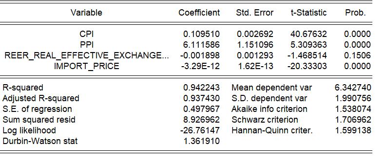
REER+B2 IMP+ B3 PPI+B4 CPI+E
Independent variable ERPT is represent exchange rate pass through. Dependent variable REER represents real effective exchange rate, IMP represents import price, PPI represents producer price index, CPI represents consumer price index.
4.3
2011 46.670 101.18 4.75304E+11 108.91 9.5% 2012 53.437 92.69 4.99989E+11 119.24 7.2% 2013 58.598 93.18 4.81686E+11 131.18 7.3% 2014 61.030 88.99 4.72434E+11 139.92 5.2% 2015 64.152 98.71 4.09237E+11 146.79 -2.5% 2016 67.195 101.99 3.7609E+11 154.05 -2.5% 2017 65.122 102.07 4.52241E+11 159.18 4.3% 2018 68.389 105.83 5.18779E+11 165.45 3.0% 2019 70.420 100.59 4.8895E+11 171.62 2.8% 2020 74.100 105.45 3.76995E+11 182.99 3.5% 2021 73.918 102.15 5.79145E+11 192.38 4.8%
ERPT=B0+B1
Empirical Results
326
Table 2: the regression between ERPT and CPI, PPI,REER,IMP in China
This is the Chinese part of the Regression, the results show that not many results show a relationship with independent variable, combined with the Chinese information shows that this is because China uses a fixed exchange rate, the state has a strict control of the exchange rate, so even if the number of imports increase, inflation continues, cannot be obvious under the exchange rate development is reflected.
On the contrary, the results in India are quite different. As in the Chinese part, the r square reaches 94% and 84% respectively showing an extremely strong credibility, and since India adopts a floating exchange rate model, it can be seen through this regression that the transmission of exchange rate changes and cpi, ppi, and imp are significantly linked, with the most influential being imp, followed by ppi, and the relatively least cpi inflation.
First, the exchange rate does matter for domestic inflation. Second, the three prices respond differently to ERPS shocks. The response is that IMP is the largest, followed by PPI and CPI is the smallest. Import price content
The IMP is the highest and the CPI is the lowest, which is a reasonable result. This finding is also consistent with previous studies such as McCarthy (2000), Hahn (2003) and Faruqee (2006) which examine exchange rate pass-through countries in Europe. 3. The price response to the ERPS shock is significantly positive. Even in the crisis period, the degree of response varies from country to country. As discussed by Burstein, Eichenbaum, and Rebelo (2002, 2005), the degree of CPI inflation following a sharp depreciation depends on (i) the extent to which imported inputs are used for domestic production and (ii) the presence of distribution costs. The impact of exchange rate shocks on domestic prices in our current analysis is closely related to the
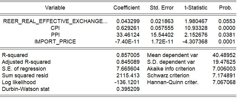 Table 3: the regression between ERPT and CPI, PPI,REER,IMP in India
327
use of imported inputs. The degree of pass-through of the exchange rate is highest in IMP and lowest in CPI, since imports are imported using the largest IMP and the smallest CPI.
5.0 Conclusion
Based on the results of the regression analysis, it can be concluded that the relationship between exchange rate transmission and inflation varies according to the exchange rate regime and import composition and varies from country to country. In China, which has a fixed exchange rate regime, changes in import prices, producer prices and consumer prices do not have a significant impact on inflation. In contrast, in India, which has a floating exchange rate, there is a strong association between exchange rate changes and inflation, with import prices having the largest effect, followed by producer prices and consumer prices having the smallest effect. These findings are consistent with previous studies and underscore the importance of understanding the specific economic conditions and policies of each country when analyzing the relationship between exchange rates and inflation. In addition, the results show that exchange rate transmission is highest Import prices, reflecting the fact that imports are heavily dependent on foreign currency and therefore more sensitive to exchange rate fluctuations. On the other hand, the degree of pass-through is lowest for consumer prices, indicating that domestic prices are less affected by exchange rate changes. This finding is consistent with the theory that the degree of pass-through depends on the extent to which imported inputs are used in domestic production and the presence of distribution costs.
Overall, these findings have important implications for policy makers, especially in countries with floating exchange rate regimes. They argue that exchange rate movements can have a significant impact on domestic inflation and that policies aimed at stabilizing the exchange rate may also help to control inflation. Moreover, the results underscore the importance of understanding each country's specific economic conditions and policies when analyzing the relationship between exchange rates and inflation.
328
BIBLIOGRAPHY:
Belaisch, A., 2003, “Exchange Rate Pass-Through in Brazil,” IMF Working Paper, WP/03/141, International Monetary Fund.
Burstein, A., M. Eichenbaum and S. Rebelo, 2002, “Why Are Rates of Inflation So Low After Large Devaluations?” NBER Working Paper 8748, National Bureau of Economic Research.
Burstein, A., M. Eichenbaum and S. Rebelo, 2005, “Large Devaluation and the Real Exchange Rate,” Journal of Political Economy, 113(4), pp.742-784.
Campa, J. M. and L. S. Goldberg, 2005, “Exchange Rate Pass Through into Import Prices,” Review of Economics and Statistics, 87(4), pp.679-690.
Campa, J. M., L. S. Goldberg and J. M. González-Mínguez, 2005, “Exchange Rate Pass-Through to Import Prices in Euro Area,” NBER Working Paper 11632, National Bureau of Economic Research.
Caporale, Cipollini and Demetriades, 2005, “Monetary Policy and the Exchange Rate during the Asian Crisis: Identification through Heteroscedasticity,” Journal of International Money and Finance, 24, pp.39-53.
Central Bank of the Republic of Turkey, 2001, Annual Report, downloaded from the web site of the Central Bank (http://www.tcmb.gov.tr/yeni/eng/).
Choudhri, E.U. and D.S. Hakura, 2006, “Exchange Rate Pass-Through to Domestic Prices: Does the Inflationary Environment Matter?” Journal of International Money and Finance, 25, pp.614-639.
Elliot, G., T. J. Rothenberg and J. H, Stock, “Efficient Tests for an Autoregressive Unit Root,” Econometrica, 64, pp.813-836, 1996.
Faruqee, H., 2006, “Exchange Rate Pass-Through in the Euro Area,” IMF Staff Papers, 53(1), pp.63-88.
27
Goldberg, L.S. and J.M. Campa, 2006, “Distribution Margins, Imported Inputs, and the Sensitivity of the CPI to Exchange Rates,” NBER Working Paper 12121, National Bureau of Economic Research.
Hahn, E., 2003, “Pass-Through of External Shocks to Euro Area Inflation,” Working Paper, 243, European Central Bank.
329
Ito, T., 2007, “Asian Currency Crisis and the IMF, Ten Years Later: Overview,” Asian Economic Policy Review, 2(1), pp.16-49.
Ito, T. and K. Sato, 2006, “Exchange Rate Changes and Inflation in Post-Crisis Asian Economies: VAR Analysis of the Exchange Rate Pass-Through,” NBER Working Paper 12395, National Bureau of Economic Research.
Kamin, S.B. and J.H. Rogers, 2000, “Output and the Real Exchange Rate in Developing Countries: An Application to Mexico,” Journal of Development Economics, 61, pp.85-109.
Kim, S. and N. Roubini, 2000, “Exchange Rate Anomalies in the Industrial Countries: A Solution with a Structural VAR Approach,” Journal of Monetary Economics, 45, pp.561-586.
Kim, Y. and Y.-H. Ying, 2007, “An Empirical Assessment of Currency Devaluation in East Asian Countries,” Journal of International Money and Finance, forthcoming.
Leigh, D. and M. Rossi, 2002, “Exchange Rate Pass-Through in Turkey,” IMF Working Paper, WP/02/204, International Monetary Fund.
McCarthy, J., 2000, “Pass-Through of Exchange Rates and Import Prices to Domestic Inflation in Some Industrialized Economies,” Staff Reports, 111, Federal Reserve Bank of New York.
McLeod, R. H., 2003, “Towards Improved Monetary Policy in Indonesia,” Bulletin of Indonesian Economic Studies, 39(3), pp.303-324.
Mihaljek, D. and M. Klau, 2001, “A Note on the Pass-Through from Exchange Rate and 28
Foreign Price Changes to Inflation in Selected Emerging Market Economies,” BIS Papers, No.8, pp.69-81.
Mishkin, F.S. and M.A. Savastano, 2000, “Monetary Policy Strategies for Latin America,” NBER Working Paper 7617, National Bureau of Economic Research.
Olivei, G. P., 2002, “Exchange Rates and the Prices of Manufacturing Products Imported into the United States,” New England Economic Review, Federal Reserve Bank of Boston, First Quarter, pp.3-18.
Otani, A., S. Shiratsuka and T. Shirota, 2005, “Revisiting the Decline in the Exchange Rate Pass-Through: Further Evidence from Japan’s Import Prices,” IMES Discussion
330
Paper No. 2005-E-6, Institute for Monetary and Economic Studies, Bank of Japan.
Parsley, D. C., 2004, “Pricing in International Markets: a Small Country Benchmark,” Review of International Economics, 12(3), pp.509-524.
Parsons, C.R. and K. Sato, 2006, “Exchange Pass-Through and Currency Invoicing: Implications for Monetary Integration in East Asia,” The World Economy, 29(12), pp.1759-1788.
Taylor, J., 2000, “Low Inflation, Pass-Through, and the Pricing Power of Firms,” European Economic Review, 44, pp.1389-1408.
Toh, M-H and H-J Ho, 2001, “Exchange Rate Pass-Through for Selected Asian Economies,” Singapore Economic Review, 46(2), 247-273.
331
