The Geology of El Paso
1
William Cornell, Diane Doser, Richard Langford, Joshua Villalobos, Jason Ricketts
i TABLE
FRONTISPIECE GEOLOGIC TIMESCALE ERROR! BOOKMARK NOT DEFINED. CHAPTER 1 - INTRODUCTION 1 CHAPTER 2 GEOLOGIC TIME AND STRATIGRAPHIC PRINCIPLES 14 Relative Time 14 Transgressions and Regressions 16 Absolute Time 22 Radioactive Decay 22 Half Lives 23 Measuring Isotopes 23 Closure Temperature 25 Absolute Dating Techniques 25 CHAPTER3 BENDING AND BREAKING -- DEFORMING EL PASO ROCKS 30 Strike and Dip 30 Folds 31 Fractures 33 Faults 33 CHAPTER 4 EARLIEST DAYS IN EL PASO 39 The Oldest Rocks The PreCambrian 39 El Paso’s Precambrian Rocks 41 CHAPTER 5 PALEOZOIC ERA 50 The Paleozoic an Overview 50 The Passive Margin and the Sauk Transgression 51 Bliss Sandstone 51 El Paso Group 53 Thunderbird Island 58
OF CONTENTS
ii The Tobosa Basin 58 The Mid Ordovician Unconformity 59 The Montoya Group 60 Fusselman Dolomite 62 The Devonian: The Canutillo Formation and Percha Shale 63 The Mississippian – Pedregosa Basin 65 The Ancestral Rockies Orogeny – Pennsylvanian and Permian 68 La Tuna Formation 69 Berino and Bishops Cap Formations 70 Panther Seep Formation 71 Permian Hueco Group 71 CHAPTER 6 MESOZOIC ERA 73 The Sevier Orogeny and the Cretaceous Interior Seaway 85 The Laramide Orogeny 86 CHAPTER 7 -- THE CENOZOIC ERA 88 The Laramide Orogeny Continued 88 The Great Ignimbrite Flare up 90 Early Rift Extension 92 The Rio Grande Rift 93 Rift Sediments 95 The Rio Grande 96 CHAPTER 8 100 FIRE AND LAKES – EL PASO IN THE PLEISTOCENE 100 Volcanos 100 Maar Volcanos 103 CHAPTER 9 107 EARTHQUAKES, FAULTS AND THE SHAPING OF THE EL PASO LANDSCAPE 107 Faults 113
iii The Pleistocene Pluvial lakes. 114 Incision of the Rio Grande 116 CHAPTER 10 119 EL PASO’S NATURAL RESOURCES 119 Fossil fuels 119 Precious metals 120 Other Industrial Minerals 122 REFERENCES 127
1. CHAPTER 1 - INTRODUCTION
During the "age of exploration," European natural philosophers noted that maps of the Atlantic Ocean and surrounding continents resembled pieces of a gigantic jigsaw puzzle and that the Americas looked as if they could be fitted against the shores of western Africa and Europe, forming a greatly enlarged continent (fig. 1-1) (Snider-Pellegrini, 1858). In the late 1800s, serious consideration was being given to this strange idea and a variety of lines of geologic evidence were being assembled. Alfred Wegener and Alexander duToit wrote extensively on the idea during the early decades of the 20th century. Their reconstructions of the circum-Atlantic continents showed that major features like the Appalachian Mountains of North America and the Hercynian Mountains of Europe formed continuous structures whose geologic histories were remarkably similar. Likewise, distribution of distinctive suites of fossils in South America and Africa (fig. 1-2) could most easily be explained if those land masses had been part of a larger, unified southern continent.
Evidence of late Paleozoic continental glaciation was incompatible with knowledge of glacial mechanics if the southern continents were separated by thousands of miles of open ocean, as today. If, on the other hand, the continents had been united, the glacial evidence was sensible and coherent.
In his widely used Historical Geology text, C.O. Dunbar (1962) wrote:
"The most remarkable feature of the Permian glaciation is its distribution. It was chiefly in the southern land masses and in regions which now lie within 20° to 35° of the equator. This circumstance, more than any other, has made attractive the belief in continental drift. If the southern continents were united to Antarctica until after Permian time, the glaciation may not have spread into low latitudes. A later "drift" of these continents toward the north would account, far more easily than any other means yet postulated, for the present distribution of the glacial deposits. But this premise itself is still in the realm of speculation!"
1


2
Figure 1-1. Snider-Pellegrini’s map showing his interpretation of how the continents fit together before the Noachian deluge, which he interpreted as shaping the world.
Figure 1-2. Distribution of fossils shown in Wegener's map of Pangaea. Cynognathus and Lystrosaurus were terrestrial reptiles. Mesosaurus lived in fresh-water swamps and ate fish. Glossopteris were the most common large trees within a diverse community that lived across large parts of Pangaea. U.S. Geological Survey rendering of the original.
Wegener was so convinced that he proposed the names Gondwanaland, Laurasia, and Pangaea for these land masses (fig. 1-3). In this terminology, Gondwanaland included the present continents of Africa, Antarctica, Australia, India, and South America. Laurasia was composed of Asia, Europe, and North America. Pangaea (literally "all lands") was the supercontinent of Laurasia plus Gondwanaland. In his book, "Our Wandering Continents," duToit expanded upon Wegener's basic concepts, added additional geologic detail and evidence, and suggested that Pangaea had formed during Paleozoic time and had broken into its present-day pieces during Mesozoic and Cenozoic time. As the supercontinent fragmented, its pieces drifted away from one another toward their present positions.
A grave difficulty persisted. Neither Wegener nor duToit were able to envision plausible mechanisms to cause large chunks (continental plates) of Earth crust to move about as required by their "drifting continents" model. The methods of classical geology, begun in the 1700s, were insufficient to provide an answer. With the benefit of hindsight, it is hard for many today to appreciate the frustration the "drifters" felt. Their methods provided unambiguous evidence for continental drift but offered no clues about processes and mechanisms to accomplish it. The 1930s, '40s, and '50s saw the theory of continental drift cycling from being dismissed as fantasy to being actively promoted, although the nay-sayers ("speculation" said Dunbar) had the upper hand. Geology underwent what Thomas Kuhn calls a "scientific

3
Figure 1-3. Alfred Wegener’s 1915 (Wegener, 1966) reconstruction of the drifting of the continents ( Lennart Kudling, CC BY 3.0 <https://creativecommons.org/licenses/by/3.0>, via Wikimedia Commons)
revolution" in the 1960s. New technology for obtaining geologic data and the new data thus acquired, coupled with new research styles, cut the "Gordian knot" of a driving mechanism and continental drift became the ruling paradigm.
Technology developed during World War II was redirected to other purposes during the post-war years. In addition, wartime experience of government funding for basic research changed the historic traditions of funding research solely from private sources. The combination of technology and funding triggered major advances throughout the scientific community as illustrated by the following examples.
Seismology is the study of vibrations in the earth triggered by volcanoes, earthquakes, and human-made explosions. A global network of seismographs (instruments that detect earthquakes) was established in the post-war years to monitor nuclear weapons tests. In addition to bomb explosions, these seismographs recorded earthquakes in far greater numbers and with far better accuracy than ever before possible. These new data pinpointed plate boundaries and confirmed ideas about processes at plate boundaries. Further, seismic studies led to increasingly detailed knowledge of the internal structure of the earth.
Although the earth's magnetic field has long been studied, post-war technology contributed to the study of magnetism in rocks (geomagnetism), and by extension, into the study of the magnetic field through geologic time (paleomagnetism). Paleomagnetic data have been used to determine the actual paths followed by the drifting continents.
Use of radioactive isotopes to date rocks began early in the 20th century, but these analyses were crude, costly, and slow. With more money available to support research, laboratories specializing in radiometric dating and in the study of stable isotopes, were established, analytical techniques were standardized, and additional useful isotopes were discovered.
Another post-war project that has contributed to our understanding of the earth has been the deep sea drilling project. It began as a "wild" idea - let us use oil-field technology to drill a hole through the sea floor all the way to the Moho (the seismic discontinuity that separates crust and mantle). The American Miscellaneous Society (AMSOC) agreed to sponsor the effort. It was unsuccessful in the great goal, drill to the Moho, but was successful enough to spawn other efforts that involved funding, equipment and personnel from many nations. Since this time other deep sea drilling programs, today continuing as the International Ocean Discovery Program, have contributed a wide variety of information about the age and makeup of the sea floor, and underlying sediments and crust. Contributions include an understanding of how deep circulation of water along mid-oceanic ridges controls the chemistry of the oceans. Deep sea drilling has also shown how warming of the climate can have profound effects on the chemistry of the oceans.
These programs have revolutionized our understanding of the earth. We now understand the oceans to be fundamentally different than the continents and have been able to obtain detailed records of ancient climates and tectonic events.
Our picture of the earth now is one of a multi-layered body, churned internally by heat which, in turn, powers the process formerly called continental drift. Early seismic studies revealed the basic layered structure of the earth; more modern work has refined and supplemented that information. In broadest terms, the earth consists of three layers - crust at the top, mantle in the middle, and core at the center (Figure 1-5). The crust and mantle are made of silicate rock, whereas the core is made of metal, mostly Iron and Nickel. Silicate rock is composed of minerals composed of silicone and oxygen bound to other chemical elements.
4
Isotopic dating using Carbon14 began in the 1950s and today is an invaluable tool for archaeologists, anthropologists, and geologists who work on geologic materials up to 70,000 years old.
Before World War II, a marine geologist interested in the ocean bottom had essentially the same tools for getting samples that were available to coastal navigators of the 1500s. A lead weight, smeared with grease and lowered to the sea floor, would pick up bottom sediment in the grease and hold it while the weight was pulled back to the surface. Dredges and grab-samplers intended to get larger bottom samples had remained virtually unchanged in design and function since the days of the H.M.S. Challenger Expedition (1872-1876).
Post-war technology changed that situation. Acoustic profiling (or sub-bottom profiling) was a spin-off from anti-submarine warfare. In its geologic application, machine-made sound waves are directed into sea floor sediments where they are reflected after traveling through sediment layers. Analysis of the reflected waves reveals details of the structure of the sea floor (figure 1-4) to depths of hundreds of meters beneath the water/bottom interface. It is now possible for a research vessel to make a continuous profile while under way so that tens of miles of sea bottom can be profiled in a day.

5
Figure 1-4 – Example of marine seismic profile (courtesy U.S. Geological Survey Open File Report 20091001)
Earth’s crust is divisible into two parts. Familiar to most is continental crust. This type of crust is about 40 km (24 miles) thick, thicker under mountains and thinner under rift valleys such as the Rio Grande rift. Rocks of the continental crust include all types of igneous rocks commonly buried under variable thicknesses of sedimentary and metamorphic rocks. In some areas, such as the Canadian Shield of North America, only a thin veneer of soil or sedimentary rock covers the igneous rock of the crust. In contrast, in the Gulf Coast region, tens of thousands of feet of sedimentary strata cover the igneous rock "basement." It has been calculated that if one collected statistically representative samples of continental crust rocks, melted these, and allowed the melt to cool and solidify, the resulting solid would have a composition close to granite. Hence, we speak of the continental crust as being "granitic". Continental crust extends seaward from the continent coast and underlies the regions called the continental shelf and continental slope. Including this material, continental crust covers about 44% of the earth surface.
Oceanic crust covers the remaining 56% of the earth surface. It differs from continental crust in thickness (average of 8 km (~5 miles)) and composition. Mafic igneous rocks (basalt, gabbro) are major constituents. Over most of the sea floor, these igneous rocks are overlain by sediments and sedimentary rocks. The sedimentary material is diverse in composition, some is biogenic material (shells of marine organisms), some is chemical (evaporite minerals), some is clastic or detrital sand, silt, clay transported into the ocean from land. If we determined the composition of oceanic crust as we did continental crust, we would find the oceanic crust is "basaltic." A final, and critical, difference is density. Continental crust has an average density of 2.6 g/cc while oceanic crust has a density of 3.0 g/cc.
Regardless of whether one is on land or on the sea floor, as one goes deeper beneath the earth’s surface, the weight of the overlying rocks (lithostatic pressure) increases. Some minerals respond to increased lithostatic pressure by changing their crystal structure to more compact, higher density forms. There is no halfway in the process - when the critical pressure is reached, all grains of the pressure-sensitive mineral change form together. When this happens, behavior of seismic waves traveling through the crystals changes. Specifically,

6
Figure 1-5. Diagram showing the layers of the earth. Note that the layer thicknesses are not to scale. Source Surachit, Wikimedia commons https://commons.wikimedia.org/wiki/File:Earth-crustcutaway-english.svg
seismic wave velocity increases in the more dense material, again without an intermediate or transitional phase. The result is a "seismic discontinuity." The base of the earth crust, oceanic or continental, is marked by the Mohorovičić Seismic Discontinuity, or the Moho, or the Mdiscontinuity. Mantle lies below, crust above.
Another phenomenon is associated with increasing depth beneath the earth surface: increasing temperature. Ever since humankind began underground mining, miners have been aware of the fact that the deeper you go the hotter it gets. The source of the heat is the core of the earth from which heat is convected toward the surface through the overlying mantle and crust. Raising the temperature of rocks causes them to expand, become less dense, somewhat plastic, and eventually to melt. Thus, pressure and temperature work against one another deep beneath the surface. Pressure wins the first round producing the Moho, but temperature wins the second.
Between depths of 125 km to 200 km (75 to 120 miles), high temperature causes mantle rock to become plastic and flow. As it flows, convectively (figure 1-6), it carries along the overlying mantle and crust, rafting continents about on the surface. These componentsmantle above 125 km and overlying crust - are referred to collectively as the lithosphere and the moving pieces are called lithospheric plates. The zone between 125 and 200 km is less rigid, more plastic, than overlying mantle, so seismic waves travel rather slowly through it. We speak of this zone as the asthenosphere.

7
Figure 1-6. Lithosphere, asthenosphere and plate tectonics (by J. Vigil, U.S. Geological Survey).
The contact between the mantle and the core (Figure 1-7) lies at a depth of 2,900 km (1740 miles). Here, temperature dominates. Internal seismic waves are of two basic types: "P" or primary waves and "S" or secondary waves (Figure 1-7). S-waves cannot travel through liquids. At the top of the core, S-waves vanish, indicating that the outer core must be liquid (Figure 1-7). The outer core is 2,200 km (1320 miles) thick and its base is at a depth of 5,100 km (3060 miles) (Figure 1-7). From there to the center of the earth (-6,378 km, 3960 miles), the region is called the inner core. Geophysical calculations indicate that the core, overall, is composed of metals, iron and nickel for the most part with lesser amounts of oxygen and, probably, sulfur.

The lithosphere consists of approximately 30 pieces (Figure 1-8). These pieces include seven "major" lithospheric plates (African, Antarctic, Eurasian, Indo-Australian, North American, Pacific, and South American); about a dozen "minor" plates (Caribbean, Cocos, Nazca, to list a few); and a dozen or so "mini" plates or "platelets." Each of the major plates, except the Pacific Plate, contains continental crust. Most of the continents have a shield, where the Precambrian core of the continent is exposed at the earth’s surface. This is usually flanked or surrounded by a platform, where the Precambrian rocks are buried under a thin veneer of younger sediments. Together, the stable shield and platform form a craton, or stable interior of a continent. Long-term geologic stability characterizes the cratons - no mountain building has taken place during the last few hundred thousand years.
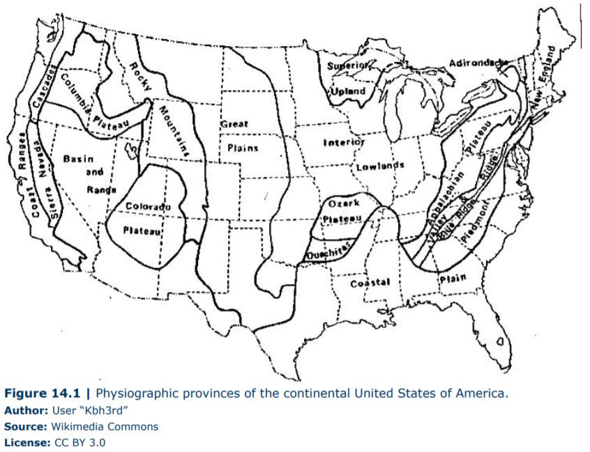
In the contiguous continental U.S. (Figure 1-9), the craton extends from the western slope of the Appalachian Plateau westward to the Front Range of the Rocky Mountains, from the southern edge of the Laurentian Shield (southern Canada) almost to the Gulf Coast. Cratons are usually more or less completely surrounded by marginal mobile belts - areas where mountain building has taken place since the beginning of Phanerozoic time or is going on today. Looking again at North America, the eastern marginal mobile belt is the Appalachian region which underwent three major mountain-building episodes (called orogenies) in Ordovician, Devonian, and Pennsylvanian time and a smaller scale deformation event during the breakup of Pangaea in the Triassic Period. Along the southern side of the craton, the
8
Figure 1-7. P and S wave velocity profiles through the earth. Note the sudden increases in the upper mantle and the loss of S waves in the outer core (Courtesy Wikimedia commons https://upload.wikimedia.org/wikipedia/commons/b/be/Speeds_of_seismic_waves.PNG).
Ouachita Mobile Belt was active during Pennsylvanian time. On the western side of North America, a series of mobile belts have developed, beginning in Devonian time with the Antler belt.

9
Figure 1-8. Map of the lithospheric plates of the earth, showing the plates and plate boundaries. Image is public domain US Geological Survey.
Figure 1 provinces of the continental United States (source: Wikimedia Commons)
Sea floor basalts are magnetized as they cool after being emplaced and they move laterally away from the MOR riding the convective circulation of the asthenosphere. As the new crust cools, it shrinks, subsides, and gradually acquires a cover of oceanic sediment. The MOR system extends for some 60,000 km (37,300 miles) around the earth and covers about 23% of the earth surface. Plates move away from the ridge at about right angles to the ridge axis at rates that vary up to 8 cm (3.2 inches) per year.
Lithospheric plate boundaries do not necessarily coincide with continent margins. The eastern margin of the North American continent lies thousands of miles from the eastern boundary of the North American plate (fig. 1-8). No tectonic (or mountain building) activity is taking place along the eastern margin of the continent, hence it is called a passive margin. On the other side, the western continental margin and the western plate margin are coincident. Tectonic activity is going on here and the margin is called an active continental margin. Lateral boundaries of lithospheric plates exhibit three basic structural styles: divergent, convergent, or transform.
Divergent plate margins are associated with Mid-ocean Ridge (MOR) (fig. 1-10) spreading centers, where mantle material is being added to the lithosphere in the form of oceanic basalt. Rift valley systems are common features of the Mid-Ocean Ridges and Rises (fig. 1-10) and may be present on continents where continental plates are being torn apart.

10
Figure 1-10 – Mid-ocean ridge (source: Wikimedia commons)
Convergent plate boundaries are regions where two lithospheric plates collide with one another. Since there are two types of crust (continental and oceanic), there are three possible types of convergent systems: continental crust/oceanic crust system; oceanic crust/oceanic crust system; continental crust/continental crust system. The critical factor which dictates behavior of the plates is the density of the crust. Continental crust is "light" (2.6 g/cc), while oceanic crust is "heavy" (3.0 g/cc), and the underlying lithosphere is even more dense. Oceanic crust varies a bit in density, generally the older it is, the denser it is.
An example of the continental crust/oceanic crust type convergent system (Figure 111a) is the boundary between the South American plate (continental) and the Nazca Plate (oceanic). The high-density oceanic plate, moving easterly from the East Pacific Rise (ridge), bends downward and is being overridden by the South American plate moving westward from the South Atlantic Ridge. The downward movement of the Nazca Plate is called subduction and the region in which this process occurs is called a subduction zone. Sea floor in the subduction zone is drawn downward, too, and a deep sea trench develops. Here it is called the Peru/Chile trench. Maximum water depths in this trench average 8,100 m (8.1 km, 4.9 miles). The subducted Nazca Plate has been driven deep into the mantle where it has been heated enough to cause melting of the oceanic crust. Molten magma is less dense than the surrounding rock, so that magma rises buoyantly toward the surface of the earth and melts continental crust as it rises. Thus the magma becomes a mix of oceanic and continental material. It may be emplaced as plutonic material in the continental crust or it may burst through to form a volcanic system. The magmas cool, forming diorite in the plutons and andesite (named for the Andes Mountains) in the volcanic regions. Friction between the two plates also causes folding and faulting in the crust, additional processes in mountain building in mobile belts. Earthquakes in the subduction zone are another manifestation of friction between the descending and overriding crust. The largest earthquakes in the world (magnitude 9+) occur in subduction zones.

11
Figure 1-11 – Three types of collision zones (a) Ocean-continent (from columbia.edu), (b) ocean-ocean (from U.S. Geological Survey), (c) continent-continent (from National Park Service)
Convergence between two oceanic lithospheric plates is the second possible situation (fig. 1-11b). The most thoroughly studied area of this sort is the Japanese Island Arc. Here again, a subduction zone is present, but the pieces are the oceanic crust-bearing stationary Eurasian Plate and the westward-moving Pacific Plate. The Pacific Plate basalts are older (and colder and denser), so this is the piece that is being subducted. Because there is no lightweight continental crust involved, there is less folding and faulting and igneous processes are more important. Throughout the Japanese islands, volcanic rocks and volcanic structures dominate the landscape. On the Pacific side, the Japan Trench (average maximum depth = 8,400 m or 5 miles) extends the entire length of the arc.

When two continent-bearing lithospheric plates collide (fig. 1-11c), their low density makes them too buoyant to be subducted into the underlying mantle. Instead, the plate edges crumple and buckle and mountains with minor volcanic components are formed. The mountain belt that extends from the Italian Alps, through the Balkans, Greece, Turkey, Iraq, Iran, Afghanistan, Pakistan, and reaches its greatest expression in the Himalayas is the product of this type of boundary system. The magnitude of this deformation is indicated by noting that the peak of Mt. Everest (8,848 m or 5.3 miles above sea level) is composed of fossiliferous mamarinemarine limestone.

12
The third type of plate boundary is the Transform margin. (fig. 1-12a and 1-12b). Along these boundaries, lithospheric plates slide past one another along transform or strike-slip faults. Because material is not rising or falling, there are usually very few volcanos along transform margins. Transform margins are most common along the mid-oceanic ridges, where they offset segments of divergent plate margins. But, transform faults may connect two segments of a MOR, they may connect two segments of a subduction zone, or they may connect a ridge with a subduction zone. One of the most famous transform margins is the San Andreas fault. The fault begins in the sea of Cortez where divergent boundaries are moving Baja California north and away from the rest of Mexico. It extends of off of the coast of northern California where it ends at another divergent margin in the Pacific Ocean. (Fig. 12b). Although folks speak of the San Andreas Fault, it, like most faults, is actually a complex of smaller, interconnected faults that collectively constitute the named fault. Through southern California, the gross trace of the San Andreas Fault trends SE to NW. On the Pacific side of the fault, gross movement is northwesterly while southwesterly motion is on the eastern side.
Because crustal material is not uniform in composition, structure, or strength, the fault twists and turns along zones of crustal weakness. In some sections, the fault displays almost constant microscopic creep, but over most of its length the San Andreas consists of "locked" segments, tens of kilometers long. Stress builds in these locked segments until the strength of the rocks is exceeded. At that point, the rocks rupture, the stored stress (energy) is released, and an earthquake occurs. In October, 1989, such an earthquake occurred, on live national television, as Americans settled in to watch the third game of the World Series. Properly called the Loma Prieta Earthquake, more than $6 billion in property damage was done in the San Francisco area alone. Near the epicenter in the Santa Cruz Mountains, the Pacific Plate moved 4 feet (1.2 m) vertically and 6 feet (1.8 m) horizontally.
Plate tectonics shape our modern landscape. California is mountainous because it is on transform and convergent margins. The Texas Gulf Coast is flat because it is not near the plate boundaries in the Atlantic and Caribbean. The rocks that we find around El Paso are the result of over a billion years of plate tectonics that has included all of the plate margins described in this chapter. Understanding how we can decipher this long history is the subject of the next chapter.
13
Figure 1-12 – a) Diagram of a transform boundary, b) San Andreas fault system (both figures from National Park Service)
CHAPTER 2 - GEOLOGIC TIME AND STRATIGRAPHIC PRINCIPLES
“The poor world is almost six thousand years old.” Shakespeare, As You Like It, act IV, scene 1
One aspect which distinguishes geological science from the other scientific disciplines is the emphasis on time. Astronomers studying distant stars and galaxies deal with ‘deep’ time (the Andromeda Galaxy, nearest neighbor to our Milky Way Galaxy, is centered about 2 million light years from earth, and galaxies hundreds of millions of light years away are known to exist). Deep time, millions and billions of years, is also the coin of geologists. For want of a formal term, we can use ‘shallow’ time as the time frame of our lives, for the time involved in laboratory experiments in chemistry and physics, for the time frame involved in most biologic processes.
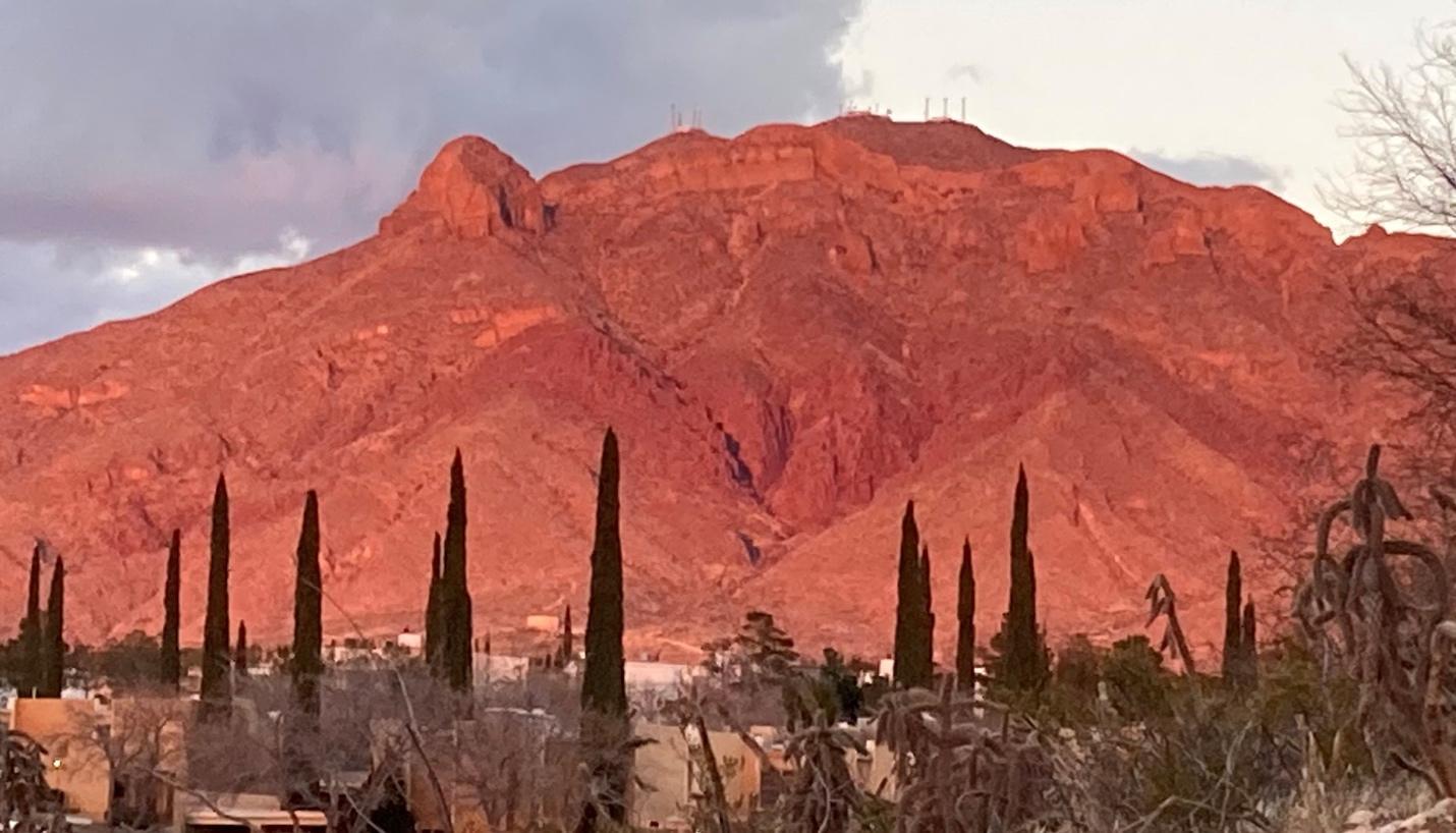
To give an example, most geologists think of the Franklin Mountains as a young and active range. It began to form about 15 million years ago. The Rio Grande first appears in El Paso about 5 million years ago, and about 550,000 years ago, it connected to the Gulf of Mexico and began to cut the valleys through which it flows today. To put this in human perspective, our species, Homo sapiens, first appears 300,000 years ago. This feature that we think of a geologically almost yesterday, is older than humanity.
Until the 1800s, scientists tended to be locked in a mindset of shallow time. Theologians had calculated that the age of the earth was approximately 6,000 years, based upon literal interpretations of all the “begats” in the Old Testament of the Judeo-Christian Bible. This notion came under fire in the scientific world with the 1787 publication of James Hutton’s book, Theory of the Earth, in which Hutton argued that the rocks of the earth contained “no vestige of a beginning and no prospect of an end.” Absence of evidence (no vestige of a beginning) is hardly proof, however. As many of the great scientists of the early 19th century were clergymen by training, mounting evidence of the earth’s antiquity made them uncomfortable. The lid blew off with the publication in 1859 of Darwin’s theory of the origin of species by natural selection. Darwin’s theory demanded a time frame for life that was Huttonian in duration and it was as clear to Darwin’s champions as to his opponents that the age of the earth was a crucial point. If evidence could be found showing a ‘shallow’ time history for the earth, then Darwin’s heresy that mankind was a highly evolved branch of the animal kingdom, rather than “fallen angels”, could be comfortably discarded. If “deep” time was available, then the Darwinian hypothesis was possible.
Relative Time
Even in Darwin’s day, a geologic time scale had been worked out. This time scale was a relative scale, meaning that, for instance, the Devonian Period was older that the Pennsylvanian Period, and that both were older than the Cretaceous Period. It was not possible, given technology of the 1800’s, to put numbers on the periods – the ages were simply “older than…” or: younger than…” ages. However, after Hutton’s book most geologists agreed, that each geologic period included a long time period.
14
This relative dating of rocks was based upon a number of fundamental geologic principles that had been articulated between 1670 and 1820. These principles dealt with the relationships of groups of rocks with one another.
The first principle, the Principle of Original Horizontally, applies to sediments and to sedimentary rocks. This says (and it is largely true) that sediments are deposited in flat layers and that if a layer has been tilted, something has happened to it.
The second principle describes the age relationships in such a sequence of horizontal sediments. The first to be deposited (layer at the bottom of the sequence) is the oldest and each layer is deposited in turn upon the previous layer. Thus, the topmost layer in the sequence is the youngest (last to be deposited). This Principle of Superposition states that in an undisturbed sequence of sedimentary rocks, the oldest bed is at the bottom and the youngest is at the top.
The third principle is called the Principle of Lateral Continuity. This says that layers of rock and sediment form continuous layers over scales of miles to hundreds of miles, and if a layer ends, something has changed.
The Principle of Inclusions says that fragments of one rock unit that are included within another are older than the rock that incorporated them. For instance, in the Franklins, the Bliss Sandstone usually sits upon the Red Bluff Granite. Red Bluff Granite fragments are found in the Bliss which means that the Red Bluff was being eroded and the fragments were being transported and deposited while the Bliss was being deposited. Thus, the included fragments are from the older of the two units. Note, however, that only relative age is indicated: Red Bluff Granite is older than Bliss Sandstone. Similarly, the Red Bluff Granite contains fragments of older metamorphic rocks as inclusions within it.
The Principle of Cross-Cutting Relations says that when one geologic feature cuts through another (a fault splits a rock layer, or an igneous dike or sill is embedded in another rock layer), the feature which cuts through is the younger and the one divided is the older.
Hutton is also credited with another important observation. At Siccar Point in Scotland, Hutton observed that beds of the "Old Red Sandstone" (now known to be of Devonian age) were deposited on top of other sedimentary rocks that stand almost vertically. Figure 2-1 is a photograph of this geologic setting. The vertical beds are now known to be of Silurian age.
Hutton couldn't tell the geologic ages of the rocks, but he concluded that they must have been quite different. His reasoning was essentially this. The vertical beds are sedimentary rocks that were laid down horizontally (Principle of Horizontality). After their disposition, they were tilted into the vertical position (a process which took some deep time). After they were tilted, erosion beveled them off to produce a flattened surface at right angles to the original bedding (another deep time-consuming process). Finally, the sediment of the Old Red Sandstone was deposited on the beveled surface. The beveled surface is called an unconformity, a break in the chronologic record of the rocks due to some combination of nondeposition or erosion. The Siccar Point example is an angular unconformity on in which the beds above and below the unconformable surface lie at an angle to one another. A substantial period of deep time separated the rocks across the unconformity.
Subsequently, two additional types of unconformities have been recognized. They are called "nonconformities" and "disconformities". A nonconformity is one in which sedimentary rocks were deposited upon plutonic or metamorphic rocks. Plutonism and metamorphism are both processes of the deep interior of the crust while sedimentation is a surface phenomenon. To produce a nonconformity, plutonic or metamorphic rocks must be formed. After their formation, the thick overlying crust must be eroded away (requiring deep time) before they are
15
exposed on the surface where they can be re-buried in sediment. Thus, the sedimentary rock must be significantly different (younger) in age than the igneous or metamorphic rock. The Red Bluff Granite/ Bliss Sandstone contact in the Franklins is a marvelous example of a nonconformity between plutonic (Red Bluff) and sedimentary (Bliss) rocks.
(https://upload.wikimedia.org/wikipedia/commons/6/6d/Siccar_point_red_capstone_from_above.jpg)
Disconformities are trickier because they form in sequences of sedimentary rocks deposited parallel to one another. To produce a disconformity, the general sequence of events is this: deposition of one unit ends, followed by either a period of nondeposition or erosion occurs, then deposition of a second unit occurs leaving two layers separated by a surface that includes missing time. Most geologists believe that the visible rock record shows us only about 10% of the time it includes. Often the two rocks will display different lithologies – one may be, a sandstone and the other a limestone - in which case an alert geologist will suspect that an unconformity is present. We will look at why said geologist might be suspicious in a bit. In other cases, lithology of both rocks could be the same – two limestones, two shales, etc.and more subtle evidence would have to be found to recognize the unconformity.
Transgressions and Regressions
Why did our alert geologist suspect a disconformity when the beds were sandstone and limestone? The answer involves another geologic principle, articulated during the 20th

16
Figure 2-1 Siccar Point Scotland. Note vertical layering on right and gently dipping layering of Old Red Sandstone at left.
century. Walther's “Law” says that sedimentary facies that are stacked in order, without an unconformity, must have formed in environments that were adjacent.
Examine Figure 2-2. In Figure 2-2, a cross section along a coast is shown. Inshore, where wave energy is greatest, only large (heavy) sediment particles will remain while smaller, lighter ones are winnowed out and carried further offshore. The result of this process is development of bands of different sized sediments, called sedimentary facies, coarse sediment (sand) in shore and finer sediment (lime mud) off shore. Suppose that we lower sea level (Figure 2-2-bottom-middle layer). The facies will shift laterally but will remain in the same order. And lower sea level again (Figure 2-2-bottom-top layer). Facies shift again, keeping the same order. From bottom to top of Figure 2-2-bottom, we see the same sequence of facies vertically that existed laterally during sedimentation in the area. In this example, sea level is falling (or "regressing" off the land) producing a regressive sedimentary sequence. Notice that the vertical progression of facies is from mud (fine) at the bottom to coarse (sand) at the top. The same sort of thing would have happened if we had been raising sea level in our example (Figure 2-2-top), but the facies would have migrated in the opposite direction and the vertical sequence would have been from coarse-grained sediment at the bottom to finer-grained sediment at the top, the characteristic pattern of a "transgressive" sedimentary sequence.
As alert field geologists, we would expect vertical sedimentary facies to change according to Walther's Principle. Finding a limestone and a sandstone vertically next to one another is contrary to the principle, and our suspicions ought to be aroused that something is not as it should be. A disconformity is one possible explanation for the violation of Walther's Principle; another possible explanation might be that a bedding plane fault lies between the sandstone and limestone and that one of the units has been displaced by fault movement.

17
Figure 2.2 The shifts in facies resulting from a marine transgression (a) and regression (b). Source (https://commons.wikimedia.org/wiki/File:Offlap_%26_onlap_EN.svg)
The final fundamental principle is the Principle of Fossil Succession, it states that in an undisturbed sequence of sedimentary rocks, fossils occur in an ordered sequence that does not repeat itself. In other words, life has evolved during earth history and the changes in the earth's biota through time are recorded in the rocks. Our concept of fossils is a rather broad one, from dinosaur bones, sharks' teeth, shells of invertebrate animals, to petrified wood. All of these are perfectly good examples of fossils, but other sorts of things are equally valid.
Our definition of a fossil is: evidence of pre-existing life. The teeth, bones, shells, etc., above, all are evidence of pre-existing life and are called "body fossils". Other examples of evidence include tracks, trails, and burrows made during life activity of organisms. Such fossils are called ichnofossils, or trace fossils. A wide variety of trace fossils have been discovered and, occasionally, at one end of a trace fossil is the body fossil of the trace-maker. Another trace fossil is a coprolite, fossilized fecal matter produced by an animal. Size and shape of coprolites indicate something about the size of the animal that produced them. More thorough examination may yield clues about the diet of the coprolite-making animal just as careful examination of a modern owl pellet reveals the animals in the owl's diet.
Microscopic animals can also make fossils. Shells of single-called plants (algae) called diatoms (Figure 2-3) can accumulate on the sea floor and be lithified into diatomite (or diatomaceous earth) which has a variety of commercial uses. A big diatom shell is approximately 1/10 mm in diameter (100 microns); most are closer to half that size. Chalk, a common sedimentary rock in the Mesozoic and Cenozoic eras, is composed of the calcium carbonate shells of amoeba-like marine protozoans called foraminifera (Figure 2-3) and of coccoliths, the shell plates produced by another group of marine algae.
Palynomorphs (pollen or spore fossils), however, have surprising fossil records. Humans are familiar with pollen produced by flowering plants, with spores produced by ferns and by mushrooms and other fungi. Many El Pasoans have seen a non-bearing mulberry tree in the spring shedding huge amounts of pollen – the yellowish cloud produced when a lowercovered branch is shaken. Each particle in that cloud is a pollen grain. Pollen grain walls (exines) are among the chemically toughest substances produced by li ving organisms. Boiling pollen grains in alkali or in mineral acids destroys the pollen contents but leaves the wall undamaged. Pollen and spores, as well as cysts of similar material produced by dinoflagellates and other algae, come through these treatments unscathed and are abundant in the fossil record.
Plant material may also be preserved as fossils, such as Petrified Forest of Arizona. A bit of "geo-trivia- is the fact that petrified palm wood is the state stone of Texas. Leaves, stems, flowers, and other plant parts can be preserved under favorable conditions and provide invaluable evidence about the composition of ancient plant communities.
The fossil record of life on earth is incomplete. We usually talk of two prerequisites of fossilization: the organism must possess resistant body parts, such as teeth, bones shells, etc.; and, following death, the remains must be rapidly buried in protective sediment isolating the remains from scavengers and preventing physical destruction. Where the organism liv es and dies obviously important. Land-dwelling organisms tend to have a poor fossil record because quick postmortem burial is unlikely. Aquatic organisms have better chances of being preserved since their bodies may sink to the bottom where burial can take place. Even more likely to be preserved are benthic organisms (clams and oysters, for example) which actually live in or on the bottom sediments. Just being benthic is not guarantee of fossilization, however. Organisms which lack resistant body parts are unlikely to be preserved, no matter where they live.
18
Also, parts are only parts. Some of the most useful Paleozoic fossils are microfossils called conodonts (cono=cone + dont=tooth) (Figure 2-4). They may be found singly or in sets. They are made of the same material as teeth and show growth bands, suggesting they are body parts of an animal; the fact that they occur only in marine sedimentary rocks indicates that the conodont animal was marine; they are found in sandstones, shales, and limestones which suggests that the animal was independent of the bottom and must have been nektonic (free swimming) or planktonic (passive floater). The nature of the conodont animal was unknown and was debated for more than 100 years. But finally, in 1983 the answer was found. The conodont animal was a small, eel like, backbone-less, creature whose only "hard" parts were the conodonts. They are now believed to be the first vertebrates, and the oldest ancestors of fish.
All fossils are not equally valuable as indicators of geologic age. Some, such as living brachiopods of the genus Lingula, have lengthy fossil records. Fossilized shells identical to modern Lingula occur throughout the Phanerozoic sedimentary rock pile all the way back to the Cambrian. Since the mere presence of macroscopic shelled fossils in a rock tells us that the rock is Phanerozoic, the identification of Lingula adds little to our information about the age of the rock. On the other hand, Lingula still live in the same sandy coastal environments they inhabited in the Cambrian, and are a very good indicator of environment. Similar fossils that occur in association with specific sedimentary facies, reflect the fact that in life these organisms were confined to specific biologic environments.

19
Figure 2-3 Foraminifera from beach sands of Myanmar. Photo from https://commons.wikimedia.org/wiki/File:Foraminif%C3%A8res_de_Ngapali.jpg#file. Under Creative commons CCU license.)
(https://www.biodiversitylibrary.org/pageimage/40483030
The fossils that are most useful for determining relative ages of rock are called index or guide fossils. An ideal index fossil possesses four attributes:

1) It has short geologic (stratigraphic) range;
2) It has broad geographic range;
3) It is relatively abundant; and
4) It is easy to identify.
By short stratigraphic range, we mean that the organisms evolved rapidly, and either evolved into another species or went extinct after only a short time. The best index fossils existed for geologically short periods of time - sometimes less than a million years. Broad geographic range means that the organisms were widely dispersed around the earth. We
20
Figure 2.4. Conodonts of the Glen Dean Formation, Chester. From Biodiversity Library.org
might find the same species in sedimentary rocks in Europe, Africa, Asia and the Americas. Living organisms that exhibit this broad geographic distribution are most frequently planktonic or nektonic marine species, species that swim or float across the oceans. Land dwelling plants and animals are usually restricted in their distribution to specific climatic regions or specific narrow eco-zones, and cannot easily cross open oceans. Benthonic marine organisms, animals that live on the sea floor, are also frequently restricted to limited environments.
(Raney Creek Member, Slade Formation, Upper Mississippian; Bighill Mountain roadcut, south of Bighill, Kentucky, USA) (30801737987).jpg, originally posted to “
by James St. John at https://flickr.com/photos/47445767@N05/30801737987).
Ease of identification is the final attribute of the 'ideal' index fossil. This is a subjective attribute because most paleontologists are specialists, expert with a small number of groups of fossils and only slightly better informed about most others. A brachiopod specialist might be able to identify at a glance several dozen species of Lingula, while a diatom specialist might be tempted to say that all species of Lingula look the same. There are some index fossils that just about every paleontologist would recognize – the Mississippian bryozoan Archimedes (Figure 2-5) comes to mind. Trilobites are definitive markers in rocks of Cambrian and Ordovician ages. Eurypterids are common in rocks of Silurian age, absent in older ones, uncommon in Devonian rocks, and rare in Mississippian to Permian ones. Fusulinids are valuable index fossils in rocks of the Pennsylvanian and Permian systems. The Devonian Period, for instance, is called the "Age of Brachiopods," the Mississippian the "Age of Crinoids”.

21
Figure 2-5. Mississippian fossils including the screw-shaped Archimedes, a bryozoan. Bryozoan are common in the oceans today. Surrounding it are clam-like brachiopods, common fossils, and still found in the oceans today. Photo from wikicommons (Archimedes sp. (fenestrate bryozoan)
Flikr”
Absolute Time
Radioactive Decay
All of the above principles were used to establish the relative ages of different rocks. Between about 1750 and 1850 all of the geologic periods we recognize today were established. Subdivision into finer time increments (epochs) has, understandably, taken longer. It is important to remember that this geologic time scale is a relative scale, one which indicated the correct order of geologic periods – Cambrian is older than Ordovician, Ordovician is older than Silurian, etc. Two of the vexing problems facing the 18th and 19th century geologists were the question of the age of the earth, in real units – years – and the question of real age for the rocks, also in units of real time – years, centuries, millennia.
In 1896, the French physicist Antoine Henri Becquerel discovered the process known as radioactivity, for which he subsequently received the Nobel Prize in physics. Recall the radioactivity is the spontaneous disintegration of the nucleus of an unstable of radioactive atom such as Uranium (U235), Potassium, (K40), or Carbon (C14). Consider the element Carbon. Carbon atoms consist of a nucleus of 6 protons and a variable number of neutrons plus a "cloud" of 6 electrons orbiting around the nucleus like a tiny planetary system around a star. The number of protons gives Carbon its chemical properties, how it interacts with other atoms. The electrons control its electrical charge and how it bonds with other atoms. The number of neutrons does not affect the chemistry of the atom, but determines its mass, or relative weight. Carbon atoms may have 6, 7 or 8 neutrons in their nuclei. Since a neutron and a proton each are about 1 atomic mass unit (amu) in weight, Carbon atoms may have masses of 12 (6 proton (p) amus plus 6 neutron (n) amus), or 13 (6 p + 7n), or 14 (6 p + 8 n). Because each of the different-mass Carbon atoms has the same chemical behavior, they are called isotopes (iso = same plus tope = activity). In the most formal usage, a Carbon atom would be designated 6C12, but since all Carbon atoms have 6 protons, we routinely shorten this to C12 . Most isotopes are stable, however, those with too many extra neutrons become unstable and undergo radioactive decay
There are four different ways in which atoms undergo radioactive decay. 1) Alpha decay involves two neutrons and two protons being ejected from the atom. This reduces its atomic weight by four, and its atomic number by two, changing it to a different element. For example, Uranium-238 decays to Thorium-234. Uranium isotopes all have 92 protons, and Thorium has 90, so the decay creates a new atom with a different chemistry. 2) Beta decay involves the ejection of either a high energy electron or a positron from one of the neutrons. Ejection of an electron converts the neutron into a proton, raising the atomic number. Ejection of a positron, converts a proton into a neutron, reducing the atomic number by one. An example of the first kind of decay is the decay of Carbon-14, which is converted to Nitrogen14, Carbon has six protons, and Nitrogen has 7. An example of the second kind of decay is Magnesium-23, which decays to Sodium-23. Magnesium has 12 protons and Sodium has 11. 3) Gamma decay usually occurs just after a beta decay; the atom has excess energy and releases it by emitting a super high energy photon, or gamma radiation. Gamma radiation is even higher energy than X-rays. 4) Electron capture is similar to beta decay, where a proton is converted to a neutron. However, in this case, the atom does this by capturing an electron to combine with the proton. An example of electron capture is the decay of Potassium-40 to Argon-40. Potassium has 19 protons and Argon has 18.
22
Half Lives
Of the 36 radionuclides, or unstable isotopes that occur naturally on earth, not all are useful for dating rocks. Some decay too quickly, and are used up within a few years. For example Tritium (H3) is almost completely gone from water within 60 years, and thus is only useful for dating very young groundwater. Therefore, radioactive decay must occur slowly enough that it occurs over geologic time scales.
We measure the rate of radioactive decay using its half-life. Radioactive decay is a random process. The time of decay of a particular atom cannot be predicted. However, in a typical mineral, there are millions of radioactive atoms, and therefore, we can use the average time for half of them to decay, which can be measured very accurately. Half-life is the amount of time it takes for half of the radioactive atoms (parent material) in a sample to decay to daughter material. For example, if a sample contains 1,000 atoms of U235, it will take 710,000,000 years for 500 to decay. Seven hundred and ten million years is the half-life of U235!"#$"%&'()"$*+,"*-&$.,/"012"34((4&-"5,*/6"7&/"892":;"&7"$.,"922<"$&"),=*5>"*-&$.,/"012" 34((4&-"5,*/6"7&/"189"3&/,":;"&7"$.,"/,3*4-4-?"892<"$&"),=*5@"*-)"6&"&-"'-$4("$.,"(*6$"*$&3"4-" $.,"&/4?4-*("6*3A(,"),=*5,)!"B.,"-'3C,/6"%&'()"(&&+"(4+,"$.46D"1222E922E892E189EFG"&/" F0EHH"&/"HIE1F"&/"10EG"&/"JEI"&/"9E8"&/"HE1"&/"8E2"&/"1E2!"K*=."LEM"/,A/,6,-$6"1".*(7 (47,@" *-) 4-"$.46",O*3A(,",(,P,-"&/"$%,(P,".*(7 (4P,6"%&'()"C,"/,Q'4/,)"$&"/,)'=,"$.,"1@222"&/4?4-*(" /*)4&*=$4P,"*$&36"$&"1@222")*'?.$,/"A/&)'=$"*$&36!"R*(7 (4P,6"*/,")477,/,-$"7&/",*=."
/*)4&*=$4P,"46&$&A,!"B*C(,"8N1"4(('6$/*$,6"6&3,"&7"$.,"46&$&A,6"=&33&-(5"'6,)"4-"/*)4&3,$/4=" )*$4-?"&7"?,&(&?4="3*$,/4*(6!
Table 2-1: Common parent and daughter isotopes used in dating of geologic materials. b.y. is billion years, m.y. is million years
Measuring Isotopes
How is the time since a rock formed measured? Most radioactive isotopes are found in minerals. Through many years of laboratory measurements, it has been learned that elements can leak in and out of minerals when they are hot. Once a mineral cools enough, the parent atoms are locked into place, and the radiometric clock begins to tick, with parent atoms
23
Parent Isotope Daughter Isotope Half Life Uranium 238 Lead 206 4.5 b.y. Uranium 235 Lead 207 710.0 m.y. Thorium 232 Lead 208 13.9 b.y. Samarium Neodymium 106 b.y. Rubidium 87 Strontium 87 50.0 b.y. Potassium 40 Argon 40 1.5 b.y. Carbon 14 Nitrogen 14 5,730 y.
decreasing in abundance and daughter products increasing over time. Therefore, it is key to be able to understand what the original amount of a radioactive element was in the mineral at the time it was “locked-in”. There are two ways this has been done. Some radioisotopes have unique daughter products that only form through radioactive decay. Others have a measurable ratio to a different isotope to the parent or daughter atom.
If a unique daughter atom does not normally occur in a mineral, then all the accumulated material had to form since the crystal cooled. The only source of Lead 206 is decay of Uranium 238. Lead 207 is the unique product of decay or Uranium 235. Therefore, by measuring the ratio of Uranium 238 to Lead 206, we can determine the age of the crystal. For example, a mineral that contains 2 parts per million of Uranium 238 and 1 part per million of Lead 206, has lost 1/3 of its original Uranium 238. Since Uranium 238 has a half-life of 4.5 billion years, this crystal cooled 2.63 billion years ago.
An example of using the ratios of parent or daughter products is Lead/Lead dating. Lead is one of the most stable elements in the earth. It does not decay and it also finds its way into many minerals. The Lead 208 that is found on the earth was there at the beginning. However, over the earth’s history, Lead 206 and 207 have increased in abundance as Uranium has decayed. All the Lead isotopes behave the same, and so the Lead locked into a crystal has the ratio that was present at the time it formed. Because Uranium 235 and Uranium 238 decay at different rates, the ratios of Lead 206, 207, and 208 can be used to measure the age of the crystal.
The third factor which makes certain isotopes useful in geologic dating is their abundance/co-occurrence. Potassium is one of the eight most abundant elements in the crust of the earth and even though the radioactive isotope is far less abundant than the nonradioactive isotopes of Potassium, K40 is still quite abundant. Furthermore, Potassium is a chemical agent which reacts readily with many other elements and tends to form strong ionic bonds. Its abundance counterbalances its rather long half-life. Rubidium (Rb87) has a monstrous half-life (50 billion years) and would, on that basis, seem too long-lived to be useful. Although Rb is rather rare, its chemical behavior causes it to be concentrated with Potassium. A rock to be dated using Potassium/Argon (K/Ar) techniques can, for relatively little additional cost, be dated using Rubidium/Strontium (Rb/Sr) technique. The Rb/Sr decay has an advantage over K/Ar, too. Both Rb and Sr have similar chemical behavior and are easily bound up in crystalline structures of ordinary minerals. In the K/Ar decay series, the Argon daughter product is a non-reactive (noble) gas. This gas is not chemically bound in the crystal and can leak out via any fractures in the crystal. If the K/Ar dates and the Rb/Sr dates agree, then confidence in the date is much greater that if only one date had been obtained. If they disagree substantially, more careful examination of the samples and review of the laboratory analysis should be conducted to find out why the numbers are "discordant" (in the terminology of the radiometrician). Similarly, Uranium and Thorium isotopes, while never abundant in crustal rocks, also co-occur, and are concentrated into certain minerals. Since each has a unique decay rate and a unique daughter product, a single sample may provide the raw material for three independent radiometric dates.
Our ability to measure the ages of rocks has improved tremendously as technology has improved. The isotopes we measure only differ in their weight, and so they are measured using a mass spectrometer that provides a chart of the masses of atoms in the sample. Mass spectrometers work by heating the rock until it vaporizes and turns into a plasma of charged gas particles. The charged particles are shot down a tube. In the middle of the tube, a large magnet pulls on the plasma, tugging the charged particles. Positively charged particles go one direction and negatively charged particles the other. Imaging throwing a ball with a wind trying to blow the ball sideways. A very light ball like a ping pong ball is thrown very far off to
24
the side, a heavier ball like a tennis ball, less so; balls that are the heaviest, like baseballs, will fly the straightest. A fan of detectors on the far end of the mass spectrometer measure the amount of charged particles and determine the ratios of different masses.
The first mass spectrometry techniques were developed right after the First World War, and steady improvements have created an amazing number of different types. Some are used for analyzing proteins from living organisms. Over time the amount of sample required has been reduced and the accuracy is increased. This has allowed the dating of new materials, and especially beginning in 1990, a revolution in dating of geologic materials has improved our understanding of the earth’s history. Today, the standard instrument used for geology is the Inductively-Coupled-Plasma Mass Spectrometer (ICPMS). This uses a gas, typically Argon, to entrain the vaporized samples. The use of precise laser beams to vaporize small parts of crystals at the front of the ICPMS, beginning in the 1980’s, has allowed dating of individual crystals, or even layers within individual crystals. Improvements over the years have produced a steadily more accurate geologic time scale. The numbers shown in the Geologic Time Scale (Frontispiece) are the current absolute ages for the geologic time periods.
Closure Temperature
Until the 1980’s most rocks required several 10 or 20 kilogram (22 to 44 pound) samples that were crushed to find enough datable material and therefore, most ages were “whole rock” ages, a single age for the entire rock. Refinement of the technique allowed smaller and smaller samples to be used, until samples of single minerals became possible. However, geoscientists were bewildered to find out that different minerals had different ages. Some minerals showed the rock as being older than others. Careful measurement of rocks under different conditions of heat and pressure turned this confusing aspect of radiometric dating from a “bug” into a “feature”.
The closure temperature of each mineral is different. That is the temperature at which parent and daughter products can no longer enter or exit a crystal and the radiometric clock starts ticking. Furthermore, the closure temperature of different radionuclides is different in the same mineral. For example, Argon will escape at much cooler temperatures than Potassium or Uranium. By dating different radionuclides and different minerals, the heating and cooling histories of some rocks has been determined. Because different metamorphic minerals grow under different conditions of temperature and pressure, this has allowed the reconstruction of ancient mountain belts, including the Precambrian mountains that formed the crust between New Mexico and El Paso.
Absolute Dating Techniques
Absolute dating techniques have proliferated in the last 50 years, and especially in the last 30 years. The most common are briefly described below:
Uranium Lead dating: Uranium Lead dating is used on Uranium bearing minerals in igneous rocks. The most common is zircon. Recently it has been applied to carbonate rocks, allowing dating of many sedimentary rocks and features. It works on rocks older than 1 million years.
Potassium Argon dating: This technique works on Potassium bearing minerals such as feldspar, biotite, and amphibole. It can be applied to rocks older than 100,000 years. It has been
25
applied to both igneous and metamorphic rocks. Recently K-Ar dating was used to make the first age measurement of rocks on Mars.
Argon-Argon dating: This uses a nuclear reactor to turn Potassium in the rock to Argon 39, then the rock is dissolved and the ratio of Argon 40 to Argon 39 is measured. The materials and ages are similar to Potassium-Argon, but the results tend to be more accurate.
Rubidium Strontium dating: This is used in dating igneous rocks by comparing the ratios of Rubidium to Strontium, and then comparing the ratios of Strontium 87, the daughter product, with Strontium 86. Rubidium and Strontium are found in different abundances in different minerals in the same rock, and this can allow a very confident age determination when several different minerals agree. The technique has been particularly useful in dating lunar rocks and meteorites. One interesting side effect of the Rb-Sr system has proven very useful in archeology. Because different areas often have different Strontium 87/86 ratios, and because Strontium is included in bone, the places a person or animal lived is recorded in the Strontium ratios in their bone, allowing the migrations and travel of ancient people to be reconstructed.
Radiocarbon (C14 dating): This technique is often used on organic materials thought to be less than 50,000 years old. Carbon-14 dating can be done because Carbon-14 is constantly being formed in the outer parts of earth's atmosphere. It forms when a proton in the nucleus of a 7N14, atom is struck by a cosmic beta particle (an electron). Fusion of the electron to the proton converts the proton into a neutron, thus changing the proton number of the atom from 7 to 6 and the neutron number from 7 to 8. This atom, then, is a 6C14 atom, and it is radioactive. Whereas the Nitrogen parent atom was relatively inert, the Carbon atom is chemically active and combines readily with oxygen atoms, forming CO2. Since the amount of incoming cosmic radiation is constant, the rate of formation of Carbon-14 is constant too. Mixing in the atmosphere carries the C14O2 toward the earth’s surface where the carbon dioxide molecule is taken up by plants during photosynthesis. The radioactive carbon becomes part of the plant tissue and accumulates in the plant until its concentration is in equilibrium with the atmosphere, an equilibrium which persists as long as the plant lives. Animals acquire equilibrium concentrations of Carbon-14 in their tissue by eating plants. Once the Carbon-14 bearing organism dies, exchange of Carbon-14 with the atmosphere stops and the Carbon-14 "clock" begins to run. During the first half life (5730 years), half of the 8 neutrons break down into an electron and a proton so that the atom's nucleus again consists of 7 neutrons and 7 protonsi.e., it has converted back to the 7N14 atom we began with. If Carbon-14 had a half-life measured in millions of years, it would be worthless as a dating tool because radiogenic and non–radiogenic Nitrogen is indistinguishable. The short half-life, coupled with the abundance of Carbon in organic matter (+30% by weight), means that we can count decay events rather than decay products to determine the age of the material.
Let's follow this thought via an example. Ordinary table sugar (sucrose) has the chemical formula C6H12O6, and one molecule of it would have a mass of 72 amu from C (carbon), 12 amu from H (hydrogen), and 48 amu from O (oxygen), for a total of 132 amu. One molecular weight of sugar = 132 grams and contains Avogadro's number of atoms, 3.02 x 10²³ atoms. One fourth are Carbon atoms, or 1.505 x10²³ atoms. Since only 1 x10⁻¹⁰ of Carbon atoms are Carbon-14, the 132 grams of sugar contains 1.505 x10 10 radioactive Carbon-14 atoms. During the first half live, half the carbon atoms would decay, giving an average rate of 2.5 decay events each minute. During the next half life, half of the remaining Carbon-14 atoms would decay, but the
26
average rate would be 1.25 decay events per minute. During the next half life, decay events would occur at an average rate of 0.625 per minute; in the next half-life the rate would be 0.312 per minute, and so on, with the number of decay events per unit of time as a direct indicator of the age of the organic matter. Since Carbon-14 decays rapidly not many half-lives would have elapsed before it would be impossible to detect decay events.
Because the amount of radiation from the sun fluctuates over time, and thus the amount of Carbon-14 that is produced fluctuates, to get accurate dates the radiocarbon “date” must be calibrated. This is done using dendrochronology, or the analysis of tree rings. Dendrochronology began in the southwestern United States and the University of Arizona has a whole department of dendrochronology. Trees add rings every year and they can record changes in climate. A dry or especially cold year will result in a thinner ring. Because individual trees can live several thousand years, comparing their records gives a unique pattern whereby the actual year the ring was made can be identified. For times older than the most recent several hundred years, dendrochronologists added trees that had died, and had overlapping records. They also used trees incorporated as roof beams in ancient dwellings of the Puebloan cultures in the Southwest. During the last 60 years, they have developed a tree ring record that goes back 11,000 years (“Radiocarbon Dating, Calibration & Databases | RADIOCARBON”).
The most recent calibration curve for radiocarbon goes back 48,000 years. However, because so little radiocarbon remains after 35,000 years, the practical limit is usually 35,000 to 40,000 years. One oddity of radiocarbon calibration is that a single uncalibrated radiocarbon date can have two or three comparable calendar dates. For example an uncorrected radiocarbon date of 1,150 bp (this is years before 1950), or 800 AD gives you possible corrected dates of 710 AD, 740 AD, and 760 AD.
Quantitative dating techniques including radiocarbon have exploded in their number and accuracy in the last 30 years. Many local geologic units have been re-dated, and new techniques have allowed dating of different features and units. Three of the techniques that have been used with success in the El Paso area are:
1. Fission Track dating. Fission is the splitting of Uranium-235 atoms, that creates atomic explosions and runs nuclear reactors. Some crystals, for example zircon, contain abundant Uranium, and when fission occurs, it creates visible damage tracks in the crystal. If the rock is warm, the tracks will heal, and therefore, fission track dating measures when rock have been uplifted, or erosion has put rocks close to the earth’s surface, and the minerals have cooled to 70-110 C° up to 300 C°, depending on the mineral studied. This technique has shown that the tops of the Franklin Mountains have been near the surface for 51 million years, and that therefore, while the mountains have been uplifted, relatively little erosion has occurred (Kelley and Chapin, 1997).
2. Optically stimulated luminescence (OSL). Sunlight causes defects in quartz crystals. These crystals repair themselves slowly. When subjected to a laser light, the defects flash and the number of flashes can be used to date when sands and silts have been buried. An OSL date gives us the oldest date for the White Sands at 6,700 years old (Kocurek et al., 2007).
3. Exposure dating. This measures a variety of isotopes that are created on the surface of a rock when bombarded by solar radiation. The isotopes gradually accumulate for as long as the rock is exposed to the sun. Exposure dating has been used to date flows in the
27
Potrillo volcanics west of El Paso to between 80,000 and 17,000 years old (Anthony and Poths, 1992)
Dating Sedimentary Rocks
Sedimentary rocks once were very difficult to date. However, accurate dates for them and the fossils within them have resulted in steady improvements in the geologic time scale. Originally, applying the fundamental principles discussed above has allowed dating of many rocks. Also, new techniques have allowed dating of sediments.
The principle of superposition can be used if a fossiliferous sedimentary rock (C) is found above a lava flow (B) or is cross-cut by an igneous intrusion (D) (fig 2-6). In Figure 2-6, the age of unit C is unknown, but must be younger than lava flow B and older than igneous Dike D.

This technique has been used to date many of the Neogene, and Quaternary sediments around El Paso. Many of these sediments contain volcanic ashes that allow their dating. The Rio Grande sediments that flowed into El Paso contain ashes from as far away as Yellowstone and California. These are within fossiliferous sediments and have allowed the dating of the rocks and the included fossils.
The principle of cross-cutting relations can be applied if an igneous rock mass - a sill, a dike, a pluton – was found within a sedimentary rock sequence. The age of the igneous rock would be younger than the sedimentary host rock. Finally, the principle of included fragments could be used to determine the maximum age of a sedimentary rock. For example, in Figure 2-7, a volcanic lava flow is being eroded by a stream and fragments of the lava rock are being buried in the stream sediments. Then the stream sediments are lithified to form a sedimentary rock. This sedimentary rock could not be older that the included fragments of lava rock : thus, we have a maximum age for the lithified sedimentary rock.
28
Figure 2-6. An example of how igneous units of known age, dike D and lava flow B, can be used to date fossiliferous unit C.
New dating techniques have also allowed dating of sedimentary rocks. In addition to the ones described above, radiometric dating of zircon crystals in sediments has provided maximum ages for many sediments. This can be used to estimate the sources of sediment in an ancient river or beach deposit. In complicated areas, such as northern Mexico, where the age of the region itself has been argued over, zircon dating has allowed a completely new understanding of the plate tectonics and geologic history in area the since 2010.

29
Figure 2
CHAPTER 3 - BENDING AND BREAKING -- DEFORMING EL PASO ROCKS
“O, what a world of vile ill-favored faults....”
Shakespeare
The Merry Wives of Windsor, sc. 4
In chapter 2 we learned that sedimentary rocks are deposited in horizontal layers. However, all around El Paso, all but the youngest rocks are tilted, folded and fractured. In this chapter we look at the different ways that rocks are deformed. For centuries geologists were baffled by the fact rocks could be deformed. We now know that heat and pressure can force rocks to deform in a variety of ways. Geologists classify deformation in three main classes: elastic, brittle, and ductile. Think of deformation in the form of bending a stick. When you start to bend it, the stick bends, but when you let go it recovers its initial shape. This is elastic deformation where deformation can be recovered. If you bend it too far, the stick breaks. This is brittle deformation and the deformation cannot be recovered. If the stick is thin and green, you can bend it, and if you bend it long enough and far enough, the stick stays bent. This is ductile deformation
Nature is more complex because rocks are not uniform and different layers in rocks differ in brittleness or ductility. Both pressure and temperature influence the ductility and brittleness of rocks. Hotter rocks are softer and often deform more ductilely. Rocks of the crust are under pressure that increases rapidly as depth increases, as does the temperature. Colder rocks, and rocks near the earth’s surface and under less pressure, break rather than bend. The other important point is the strength of the rock. Sedimentary rocks vary tremendously in strength, but are typically soft, and can be folded more easily than igneous rocks, which are much harder. Metamorphic rocks also vary in strength, and can be as easily deformed as sediments, or as tough as the hardest igneous rock.
Strike and Dip
When rocks are stressed, they eventually deform. You can look up at the Franklin Mountains and see that the layers of sedimentary rock are tilted up to the East and down to the West. How do we describe the orientation of beds like those in the Franklins? They can be described using strike and dip. Strike is measured using a compass direction, using the concept of azimuth. For example, if you are walking in a perfectly northeast direction, you are walking at an azimuth of 45° east of north. By using compass degrees we can be more accurate than using vague terms like northeast. Strike is defined as the direction you would be walking if to stay horizontal on the surface. For example, if I wanted to walk a strike line, I would walk on the surface of a bed without walking uphill or downhill. Figure 3-1 shows how strike and dip can be measured. If you mark a horizontal line along a surface and look at it from above, the compass direction would be the strike. Dip is the angle that a bed or other geological surface dips into the ground. A horizontal bed strikes in all directions and has a dip of 0°. A vertical bed or other surface has a dip of 90°.
30
Folds
Most often, deformation is caused by fracturing or by folding. Folding occurs through ductile deformation in rocks when they are compressed. Lay a sheet of paper on a flat surface, hold one edge in place, and push (compress) the other edge toward the first. The paper will begin to fold into arches and troughs. Figure 3-2 illustrates this sort of deformation in a layer of sedimentary rocks. The arches are called anticlines and the troughs are called synclines. At the left side of Figure 3-2 simple folds are shown, while the middle part carries the process further so that folds are beginning to collapse upon one another producing overturned folds (right side of figure). Eventually, the fold can by laying essentially flat, and is termed a recumbent fold. A spectacular example of a recumbent anticline is visible on the north face of the Sierra de Juarez in the central portion of the range, near the skyline (Figure 3-3). In synclines, the youngest beds (green beds, Figure 3-2) are in the axes of the folds and older beds (orange beds) comprise the flanks. In anticlines, the oldest beds are axial and younger beds form the flanks. Folds may be symmetrical or asymmetrical (Figure 3-2), and they may be tilted to form plunging folds (Figure 3-4).

31
Figure 3-1 Diagram showing how strike and dip are measured. Strike is the horizontal line on a dipping surface. Dip is the angle at which the surface goes down into the ground. The dip direction is always perpendicular to strike. https://openpress.usask.ca/physicalgeology/chapter/13-5measuring-geological-structures.


32
Figure 3-2 – Example of symmetrical, asymmetrical and overturned (recumbent) folds. The folded orange unit is the oldest and the green unit is the youngest. Image from opentextbc.ca
Figure 3-3. Recumbent fold visible from downtown El Paso the cliff at the top of the mountain is sharply folded at the right hand side of the mountain and forms an angled cliff beneath itself. Photo Richard Langford 2022.
Fractures
Fractures in rock may result from compressional, tensional, or shearing stresses. Joints are fractures that exhibit little movement while faults exhibit movement of centimeters to kilometers. Joints are common in igneous rocks and form when a magma or lava cools, solidifies, and shrinks. As shrinkage progresses, tension develops and the rock cracks to produce a set of joints. Usually the joints are roughly perpendicular to the surface of the igneous mass. The Devil's Postpile in California (Figure 3-5) is a dramatic example of such jointing. Such joints often have nearly vertical dips (Figure 3-5). When deep plutons are unearthed by erosion, another set of joints often forms, parallel to the Earth surface because reduced lithostatic pressure permits the rock to expand. These joints are important in the process called sheeting or spalling.

Faults
Faults tend to be linear fractures across which significant movement has taken place. Faults are classified on the basis of their geometry. The major geometric components are illustrated in Figure 3-6. The fault plane is the surface along which movement occurred; its intersection with the ground surface is called the trace of the fault. In flat ground, this is usually close to the strike of the fault. Fault planes may have horizontal dips, or vertical or anywhere in between.
33
Figure 3-4 Illustration of plunging folds. Image from openpress.usask.ca
Figure 3-5 – Devil’s Post pile showing joints due to cooling of igneous rock. Photo from Wikimedia
Looking more closely at the fault plane (Figure 3-5) notice that if the plane is not vertical, there is a rock surface above and another below the plane. The surface above is called (from old-time mining days) the hanging wall (you can hang your lantern from it) and the surface below the fault is the footwall (upon which you stand while you work). Movement along the fault planes can be in any direction, called “dip-slip," "strike- slip”, or “oblique-slip". In dip-slip motion, the rocks move parallel to the dip of the fault plane. In strike-slip motion, movement parallels the strike of the fault. Oblique-slip is at an angle, with some dip-slip and some strike-slip movement.
In dip-slip faults, the key question is which way the hanging and foot walls moved relative to one another (Figure 3-6). To understand the importance of this, put a book or some other thin flat item between your palms, then angle your hands with one hand angling above and one below. If you pull your hands away from each other a little, and keep them both on the book, the hand on top will move down. When the hanging wall moves down, rocks are being pulled away from each other. Now try to move your hands toward each other. Notice that, no matter which hand is on top, that hand will move further up on the book. In geological terms the hanging wall moves up.
When the rocks are being pulled apart, and the hanging wall moves down, the resulting fault is called a normal fault (Figure 3-6 top right). When the landscape is under compression from the sides, the resulting fault, where the hanging wall moves up, is called a reverse fault (Figure 3-6 top left). Some reverse faults are nearly flat and move rocks across great distances (10’s of kilometers), and these are known as thrust faults.
Strike-slip faults are often vertical, and in any case the hanging wall does not move up or down. Instead, rocks are displaced along the fault to one side or another. Two kinds of strike slip faults are distinguished. Imagine standing on the ground looking across a fault. If the rocks across the fault from you have been moved to your right, the fault is called a right-lateral strike slip fault. If the rocks across the fault from you have been moved to your left, the fault is called a left-lateral strike slip fault. The strike slip fault in the bottom of figure 36 is a right-lateral strike slip fault

34
Figure 3-5 – Block diagram of illustrating terms and features related to earthquakes as well as showing the parts of a fault. From earthquake.usgs.gov
These terms, normal, reverse and thrust, are also applicable to oblique-slip faults. Oblique slip faults can use combined terms for example an oblique normal left lateral fault combines those two movements In the El Paso area, all of these basic types of faults occur. The major ones are shown in Figure 3-7. Similarly, many different kinds of folds may be found. Most of these can be related to the major plate tectonic events that shaped El Paso geology during the 1.37 billion years of history recorded in the region.

Faults can also be classified historically as active (movement has taken place during historic time), inactive (no movement in historic time but movement has taken place during the last two million years), or extinct (no movement during the last two million years). Faults in El Paso are all classified as inactive. They have moved, but not historically. The fault with the most recent movement is the East Franklin Mountains fault, which has moved several times in the last 10,000 years (Figure 3-7).
Faults can be found in rocks of all ages in El Paso (End Piece Geology Map). These will be described in detail in the different chapters. However, most can generally be ascribed to the major orogenies, or mountain building events in the region.
35
Figure 3-6 – Three major types of faults. From National Park Service.
Figure 3-7 – map showing major faults and folds of El Paso area. Faults in the El Paso area are mostly classified as inactive. They have moved in the last 2,000 years, but not historically. The colors show the relative ages of the faults, with the most recent having moved in the last 10,000 years, and the rest last breaking the surface at older times. The thin red lines mark the locations of faults that have move in the latest Pleistocene (50,000 years). The blue and purple lines moved in the Late and Middle Pleistocene. Faults from USGS fault database. (https://www.usgs.gov/programs/earthquake-hazards/faults). The base is Courtesy of Google Earth Terrain.
Figure 3-8 – Schematic cross section through the Franklin Mountains showing the faults that bound them. On the East is the East Franklins Normal fault, the most active in the area. On the west side of the mountains, the West Franklin Fault zone includes a reverse fault that puts Ordovician rocks against Permian rocks (the one dipping under the mountain. and a Normal fault the puts younger Permian and Cretaceous rocks against the mountain front.
Total movement is estimated at 30,000 feet (9.1 km) on the eastern boundary fault, with the Hueco Bolson block down-dropped 9,000 feet (2.7 km). The other 21,000 feet (6.4


36
km) of displacement is determined by projecting a complete stratigraphic section up the western slope (or dip slope) of the Franklins until the Permian rocks intersect the projected fault plane. In Figure 3-8, the Eastern Boundary fault (EBF) plane dips to the east beneath the Hueco Bolson, as indicated by geophysical studies. Recent investigations (McCalpin, 2006) based on trenches dug across the EBF indicate that the EBF has experienced 3 to 4 earthquakes in the past 64,000 years. During each earthquake the ground moved about 6 feet (2 m), equivalent to a magnitude 7 event. Smaller normal faults are also found within the central Hueco Bolson (Figure 3-7). These faults have vertically offset sediments with ages less than 800,000 years old by 6.5 to 23 feet (2 to 7 m) (Collins and Raney, 1994)
The Western Boundary fault (WBF) has less displacement, about 10,000 feet (3 km), shown by displacement of the sedimentary rocks along the fault zone (Figure 3-8). Where the fault plane crops out, it dips easterly into the range at angles between 45° and 75° making it a reverse fault. However, gouge (wall rock pulverized during movement) includes rock fragments that could only have been emplaced if some normal movement occurred as well as reverse movement.
Within the Franklin Mountain block (Figure 3-8), other faults are present. Two have markedly affected the landscape. Southernmost is the McKelligon Canyon fault which cuts diagonally across the range. Near the head of McKelligon Canyon, the fault bifurcates and one branch extends north to intersect the Fusselman Canyon fault, while the other continues across the range and intersects the Western Boundary fault. McKelligon Canyon, as a physiographic feature, exists because faulting shattered rock in the fault zone, making it easily eroded. In the canyon itself, the fault trace is buried under colluvium and alluvium but offset of the rocks on either side of the fault shows that the northeastern side dropped down and the northwestern side moved up. The fault plane is nearly vertical where it passes across the crest of the range.
Fusselman Canyon, the valley in which Trans-Mountain Highway was built, is another fault-generated (or structurally guided) physiographic feature. Through Fusselman Canyon this fault trends east/west until it loops south about 0.5 mi (805 m) east of Smugglers Gap. The south loop joins the northern end of the north-trending McKelligon Canyon fault so that the two form an arcuate fault system opening into the Hueco Bolson. Stratigraphic separation indicates that the rocks inside the arc dropped down and out into the bolson while the rest of the range was being uplifted. This is now recognized as a low angle normal fault that formed early in the uplift of the Franklin Mountains and then rotated to nearly flat as the range grew
Faulting that produced the Sierra de Juarez probably began about 80 million years ago and edded about 40 million years ago. The geologic symbols that look like saw-teeth in the geologic map (Geologic Map – Forthcoming in the new edition) mark the thrust faults separating the allochthons from the autochthons and one another. Planes of these faults are almost horizontal or dip slightly to the southwest. In the map, the double-headed arrow (↔) is the symbol for an anticline and the other (→←) marks a syncline. All the rocks in the thrust sheets are Cretaceous units that were shoved to the northeast during Laramide compression. Each of the thrust sheets probably formed during separate compressional pulses. Along the southeastern side of the Sierra, the dashed line indicates an inferred fault that could be projected north to intersect the eastern boundary fault. There is no hard evidence to support such an inference. Just west of it a right-lateral strike-slip fault cuts across the range. It may have formed when the Sierra thrust sheets collided with the ancestral southern end of the Franklins. Finally, andesite was injected into the fold axes and fault planes. Since the andesite is neither folded nor faulted, emplacement must have taken place after deformation was finished. Recall that these andesites are over 50 million years old. None of the Santa Fe
37
Group sediments that cover Sierra faults are displaced, so the faults must be extinct or inactive
Another major thrust fault was found during drilling that revealed the Clint Fault. It is called the Rio Grande Thrust, and includes the same suite of rocks found in the Sierra de Juarez thrusts, and it is not exposed on the surface. It probably formed at the same time thrusting was taking place in the Sierra but evidence is too scanty to say more.
Numerous folds and faults developed at Cerro de Cristo Rey during emplacement of the Muleros Andesite. Host rocks were flat-lying Cretaceous units with a few gentle folds that pre-date the intrusion. As the andesite was emplaced, it domed the host rocks up and over the magma chamber initiating a series of radial faults extending outward like spokes on a wheel. These radial faults show only a few meters of movement. Striations and polished surfaces on the fault planes (called slickensides) are common but cannot be used to determine the amount of movement. A second set of faults developed later as the magma of the pluton cooled, shrank, sank downward, and solidified. This fault set is circumferential and almost completely surrounds the intrusion. Again, movement was not great - a few meters. Santa Fe sediments cover many parts of the radial and circumferential faults but are not displaced, again indicating that no movement has taken place on these faults during the last million years.
Close by Cristo Rey the Mesilla Valley fault trends northerly. It is a normal fault, down to the west, that can be traced from Cristo Rey toward Anthony fairly easily. Further north it is harder to follow because leveling of the land for agricultural purposes has obliterated the fault scarp. Near Las Cruces, it can be followed again for some distance. The presence of the fault scarp in the Rio Grande flood plain indicates that some movement has occurred since the Gold Hill terrace was carved. Maximum age of the fault is post-andesite intrusion (47 million years ago). Had the fault been in existence earlier, the Campus Andesite and the Muleros Andesite would have followed the shattered rock of the fault zone rather than cutting through solid country rock. Instead, the fault passes between the two plutons and is the structural guide for the Rio Grande through "El Paso del Norte del Rio Bravo," or El Paso Canyon. Evidence that it is a normal fault is found in the Finlay Limestone outcrops near the railroad bridges over the river. The top of the Finlay (before quarrying)was 200 or so feet (~ 60 m) above the river on the east bank (east side of the fault) while it is only 100 feet (30 m) above the river on the west bank, indicating that the west side of the fault dropped down.
38
CHAPTER 4 - EARLIEST DAYS IN EL PASO
"What
seest thou else
In the dark backward and abysm of time ?"
Shakespeare, The Tempest, act i, scene 2
The Oldest Rocks The Precambrian
Although we are certain that older rocks underlie the Precambrian units of the El Paso area, there are no data available to tell anything about them. However, samples from deep wells, and outcrops in the San Andres and Sacramento Mountains, tell us about how and when they formed (Adams and Keller, 1996; Barnes, 2001; Whitmeyer and Karlstrom, 2007). Most of these rocks are metamorphic rocks.
Metamorphic rocks are rocks that have been changed due to heat and/or pressure. There are two kinds of metamorphic rocks. Contact metamorphic rocks are rocks that have been altered by being heated by a nearby igneous rock, for example a granite intrusion. The heat bakes the rocks and causes new minerals to grow. Contact metamorphic rocks are usually found only within a few hundred meters of an intrusion and are thus local in extent.
Regional metamorphic rocks are rocks that have been buried deep within the earth to where they have been subjected to heat and pressure great enough that new minerals formed and the rocks have been deformed, picking up new fabrics. The most common fabric is foliation. Foliation forms when rocks are compressed and mineral grains rearrange themselves so that flat grains are generally perpendicular to the pressure and are all in alignment. This forms a new layering in the rock that might be at angles to the original bedding. If the rocks are deformed enough, all traces of the original bedding are destroyed and metamorphic foliation is the only visible layering in the rock. The oldest rocks in the El Paso region are regional metamorphic rocks and most show foliation. The Precambrian rocks include granites that have intruded meta-sediments and meta-volcanic rocks. Schists, amphibolites, quartzites and metaconglomerates are the most common rocks.
New minerals are formed during metamorphism that replace the original sedimentary or igneous minerals. Some minerals form in well-defined ranges of heat and pressure that allow a reconstruction of the temperatures and pressures they were subjected to. New advances in radiometric dating of metamorphic and igneous minerals have allowed a detailed understanding of how the North American craton was developed.
To the north and west of El Paso lies the Mazatzal Province, an area of metamorphosed sediments and granites that formed as an ancient sea was subducted under the North American craton between 1.65 and 1.6 billion years ago (Condie, 1982; Karlstrom and Bowring, 1988; Whitmeyer and Karlstrom, 2007; Duebendorfer et al., 2015) (Figure 4-1). A similar process has added much of California, Oregon and Washington to North America in the last 180 Million years. The rocks are dominantly schists and quartzites that were buried to
39
depths of 12 km to 15 km (7.5 to 9.5 miles) below mountain ranges formed along the subduction zone (Whitmeyer and Karlstrom, 2007). Temperatures varied from place to place depending on how close the rocks were to the volcanic arcs adding hot granitic magma to the crust.
There is debate as to whether the Mazatzal province was firmly a part of North America before 1.4 billion years ago. Recently, correlation of igneous intrusions and metamorphic rocks across northern New Mexico and Eastern Arizona suggests that another orogeny, the Picuris Orogeny, intruded and caused large scale metamorphism within the Mazatzal province between 1.49 and 1.4 billion years ago (Amato et al., 2011; Daniel et al., 2013). In southern New Mexico the Picuris orogeny is not evident, and the rocks are more typical of the Mazatzal Province, with ages ranging from 1.72 and 1.63 billion years old (Amato et al., 2008).
To the southeast of El Paso, the Precambrian rocks are much younger (1.55-1.3 billion years old) and are considered part of the Granite Rhyolite Province (Barnes, 2001) (Figure 41). These rocks are mostly only known from cores in deep wells because they are buried and they are dominated by metamorphosed rhyolites that are intruded by granites and mafic igneous rocks (Barnes, 2001). This part of the continent is inferred to have formed in and behind a volcanic arc, as oceanic crust was subducted under North America between 1.38 and 1.32 billion years ago (Barnes et al., 2002)
The Granite Rhyolite province is differentiated from a third province, the Grenville, or Llano province to the southeast along a line that runs just southeast of El Paso (Figure 4-1). In the Granite-Rhyolite province, the 1.38 to 1.3 billion year granites have Sm/Nd ages (remember from Chapter 2) that are significantly older indicating the original crust that the granites and rhyolites formed in was older, and similar in age to the Mazatzal Province (Whitmeyer and Karlstrom, 2007). However, in the Llano/Grenville Province to the southeast of El Paso the age of the deformation is similar to the age of the crust, meaning that in this area, the crust was being formed at this time, representing a new addition to the continent through accretion of island arcs and subduction under North America (Bickford et al., 2000; Barnes, 2001; Karlstrom et al., 2001). This means the rocks represent the formation of a new piece of the continent (Whitmeyer and Karlstrom, 2007; Davis and Mosher, 2015). These rocks are exposed west of Van Horn, TX in the Carrizo Mountains, where they crop out as highly metamorphosed sedimentary and volcanic rocks, originally deposited along a volcanic arc at the edge of the continent (Davis and Mosher, 2015) (Davis and Mosher, 2015) (Figure 4-1).
The rocks associated with the Grenville terrane were thrust back onto North America about 300 million years after they formed during what is known as the Grenville orogeny. In Texas, the rocks of the Llano Uplift and the Carrizo Mountains were both strongly deformed at this time. The Carrizo Mountain group was deformed along strike slip faults and smeared out to the northwest over thousands of kilometers, and in the middle of this smearing, they were thrust onto older rocks to the northeast (Davis and Mosher, 2015). The only place this thrusting is exposed is in the Carrizo Mountains, just west of Van Horn (Figure 4-1), where they are thrust onto much less metamorphosed rocks that probably were sediments at the time of thrusting (Mosher, 1998; Davis and Mosher, 2015). The less metamorphosed rocks on the north side of the thrust are of particular interest to us because they are the same rocks as the oldest rocks in the Franklin Mountains.
40
El Paso’s Precambrian Rocks
El Paso's Precambrian rocks are exposed in the Franklin Mountains (Figure 4-2) where they form the center of the range, flanked by younger rocks to the south and north (See Geologic Map Forthcoming in the new edition). Most of the accessible outcrops of the Precambrian are found on the eastern slopes of the range and in the road cuts along TransMountain highway, but the most spectacular outcrop is the "Thunderbird" on the west slope, south of Trans-Mountain Highway. In the Tom Mays Park section of the Franklin Mountains State Park there are additional outcrops of Precambrian rocks, including the rocks of North Franklin Peak. The Precambrian rocks are easily spotted because most are a pinkish red, as opposed to the grey of the rest of the range.

Precambrian rocks in the Franklins are either metamorphosed sedimentary rocks or are igneous rocks of several sorts. Geologists discuss rock sequences beginning with the oldest and working their way through progressively younger units. Following that pattern, the oldest rocks in the Franklins are the Castner Marble and the Mundy Breccia. These are equivalent, and similar to the Allamoore Group in the Van Horn area. The Castner Marble has been dated at 1.25 to 1.27 billion years old based on Uranium Lead dates from ash beds near the top of the Castner (Pittenger et al., 1994; Bickford et al., 2000). In the Franklins, as at Allamoore, it is interbedded with basalts and basaltic sills, and was probably deposited in a back arc basin, in a shallow and narrow sea, that did not have much access to the open ocean (Gore, 1985; Pittenger et al., 1994; Bickford et al., 2000).
The best place to see the Castner is in road cuts along Trans-Mountain Hwy, low on the eastern slope. There the Castner is approximately 1,400 feet (335 m) thick, but the true thickness of the Castner is not known. In the Trans-Mountain Highway outcrops, the exposed Castner is a huge roof pendant, a mass of country rock that was surrounded by molten granite
41
Figure 4-1 Precambrian terrane boundaries in the El Paso region.
and has essentially fallen in. There is no way to tell whether or not the entire thickness of the Castner is included in the pendant, or what rock may have underlain it. The Allamore Formation is similar in thickness and also does not expose any underlying rocks (Bickford et al., 2000). The Castner consists chiefly of marble (recrystallized limestone) with minor hornfels (metamorphosed shale) in the original bedding planes. Metamorphism has generated many minerals including garnets (sadly, not of gem quality), tremolite, serpentine, apatite, and others which make the Castner a favorite hunting ground for mineral collectors.
The oldest fossils of the El Paso region occur in the Castner. These are stromatolites whose prime architects were cyanophytes or blue-green algae. The stromatolites are roughly domed shaped structures, a few tens of centimeters to a meter or so in diameter that formed small mounds on the sea floor that form as sediment particles are trapped onto the sticky surface of the algae. Stromatolites are common in rocks in the PreCambrian, Cambrian and Early Ordovician, where they formed in areas where light could reach the sea floor. In the middle of the Ordovician the evolution of snails created a group of organisms that love to eat algae, and since that time, stromatolites have been restricted to harsh or very saline environments.

42
Figure 4-2. Road cut on Trans-mountain Road, on the east side of the Franklin Mountains showing orange granite intruding the green Castner Marble and the Black Mundy Breccia. Note the bedding in the Castner and Mundy is at different angles in different blocks. These represent the random orientations of blocks that have dropped into the molten granite as it melted and intruded into the older rocks above it. Richard Langford 2022.
Sedimentary structures are present and, also, indicate a shallow, marine shelf and intertidal depositional setting. Among the more spectacular sedimentary structures are intraclast conglomerates. These can still be found on the sea floor today where limestone is quickly hardened on the sea floor and a storm can rip up clasts that are then quickly deposited as the storm wanes. Depending upon how much churning the sediment pieces experience, their edges and corners may be only slightly rounded or the pieces may be turned into balllike objects, or something in between. Sedimentary rocks composed of well-rounded fragments in a finer matrix are called conglomerates. If the particles are dominantly angular the rock is called a breccia. In the Castner situation, almost all stages of angularity to rounding can be found in what are called intraclast conglomerates and breccias. The same storms that ripped up the sea floor deposited graded beds as the storm waned. Graded beds have coarse-grained particles at the bottom and are progressively finer grained toward the top. Also, late in the depositional process or early in the lithification process, some of the soft, limy muds deformed under their own weight and produced a variety of soft sediment deformation features.
In a few places in the Franklins, the Castner is interbedded with the Mundy Formation. The Mundy was originally thought to be younger than the Castner, but it is interbedded with the upper part of the Castner. It forms a large lens in the upper Castner, and was probably a basalt lava flow that erupted onto the seafloor (Ballard, 1997). The Mundy contains hexagonal cooling joints, which form as lava flows cool. Well defined pillow basalts are common (Ballard, 1997). Pillow basalts form when lava flows under water and the outside of the magma is frozen, making a feature about the size and shape of a bed pillow. It cracks and the lava flows out and is frozen to make another pillow. Much of the Mundy is autobrecciated

43
Figure 4-3. Stromatolite from the Castner Marble. Each of the two small dome-shaped features in the center and right side are some of the oldest fossils in El Paso. Source, Callan Bentley, Mid-Atlantic Geo-Image Collection License: Creative Commons Non Commercial
(Ballard, 1997), which is when the cooled outer surface of basalt flows crumbles as the molten lava within pushes the flow along.

Around and beneath the Mundy Breccia, the Castner was deformed, because it was mostly soft sediment (Ballard, 1997). Spectacular soft sediment folds formed around the edges of the basalt flow. These are one of the most interesting and photogenic features of the Castner.
At this point, we should discuss the beauty of these rocks. The Castner is one of the prettiest rocks in North America. It has interbeds of green and white that make it a prized “bookend” or other block. The colors are the result of metamorphism, which will be discussed in detail below. After deposition, the Castner was intruded by granite, causing contact metamorphism, but then was buried deep enough and heated enough to reach the greenschist stage. Greenschist describes a typically green metamorphic rock, formed when sediments or igneous rocks are compressed and heated so that the minerals in them are converted to new, generally green minerals. Greenschists usually form at temperatures between 300–450 °C (570–840 °F), and at depths of 2 to 10 kilometers.
The marble contains centimeter to meter thick bands that were originally limestone, and others that contained silt and clay. The limestone was turned into white marble, and the silty and clayey bands were transformed into the green minerals serpentine, tremolite, actinolite, and chlorite. The result is a really beautiful rock. Some of the Mundy was transformed into amphibolite where it was near the granite. Amphibolite is a shiny black rock that can give these pieces of the Mundy a beautiful satiny appearance.
Overlying the Mundy and the Castner is the Lanoria Formation. The Lanoria forms a prominent set of white and black bands along the east side of the Franklins. The black bands are metamorphosed siltstones and the white bands are the rock quartzite. In general, the Lanoria consists of fine-grained quartz sand, sometimes iron-stained, which is well bedded and contains ripple marks and occasional pebble conglomerates. Metamorphism has fused the quartz grains together, turning the once-sedimentary rock into quartzite. Within the Franklins, the Lanoria is up to 2,424 feet (739 m) thick. It is divisible into six stratigraphic sequences (Seeley, 1999). The Lanoria is interpreted to represent the progradation of a coastline into a subsiding basin from the south (Seeley, 1999). An initial transgression (see chapter 2 for discussion of transgressions) is overlain by a thick shale, and then a sequence of alternating shoreline sandstones and offshore shales (Seeley, 1999). The shales thicken and the sandstones thin to the north. No body fossils have been found, but trace fossils are fairly common in the finer grained sandstones and coarser mudstones (see burrows in Figure 4-4).
44
A combination of restricted access (the best outcrops of the Lanoria are in military firing ranges) and daunting cliffs have limited study of the Lanoria. No body fossils of any sort have yet been found in the Lanoria, so its age can only be inferred. It overlies the Castner and Mundy, so must be younger than those units and it is intruded by granites of the Red Bluff Granite complex so must be older than the granites. Since radiometric age dates on the granites are consistently in the 0.98 billion to 1.01 billion years the Lanoria Formation must be more than 1.01 billion, but less than 1.25 billion years old.
Intruded into, and engulfing the Castner/Mundy/Lanoria package is a complex of igneous rocks, dominated by the granites of the Red Bluff Granite. The Red Bluff Granite forms the distinctive red base of the Franklin Mountains on the east side. It is a typical granite batholith, formed when large masses of granite melt their way up into the middle of the earth’s crust. At the north and south ends of the range Paleozoic sediment rests directly on the granite. In the center of the Range, near North and South Mount Franklin peaks, Precambrian volcanics of the Thunderbird Group overlie the granite and the Castner, Mundy, Lanoria metamorphics.
The granite is classified as an “A” type granite (Roths et al., 1993; Shannon et al., 1997). This means that the granite is formed from a melt that contained little water. This type of granite usually forms within plates under extensional regimes, and the Red Bluff has been interpreted as a product of a large basalt intrusion to the crust, that gradually solidified until only granite was left. At least five distinct granite phases are present. Although their relative ages are unclear, the coarse-grained, pink, feldspar-rich granite is the largest volumetrically. Granite and rhyolite boulders of the same age and, similar in composition to the Red Bluff can be found in the Hazel Formation near Van Horn, suggesting that similar granites and rhyolites were widespread across West Texas at this time (Bickford et al., 2000)
In addition to the granite complex, another intrusive suite is present in the Franklins. This suite consists of diabase sills and dikes emplaced within the Red Bluff granites. Diabase is a fine-grained mafic igneous rock composed of feldspars and pyroxenes. Since it cross-cuts the granites, it must be younger than the Red Bluff. A similar diabase dike cuts Ordovician and Silurian sedimentary rocks elsewhere in the Franklins. While it seems likely that only one post-Silurian diabase is present, no physical connection has been found between the two dike systems and there may really be two - one Precambrian in age and the other post-Silurian. The diabases weather more easily than their host rocks, so their manifestation on the ground is usually a trench that looks as if someone had used a back-hoe to dig it. That trench acts as a natural channel for surface water run-off and directs some of it deep into the diabase to extend chemical weathering effects far into the dike.
45
Figure 4-4. Burrows (Left) and ripple marks (Right) in the Lanoria Fm. John Seeley 2002.
Sitting on top of the Red Bluff Granite is the final Precambrian unit of the Franklins. In 1909, G.B. Richardson (Richardson, 1909) published the first, and still only, complete geologic map of the Franklins. In his mapping, he recognized the Thunderbird Rhyolite, a name which stuck for more than 110 years. The name is derived from the unit's outcrop on the western slope of the Franklins above the Coronado area. Viewed from the west, the outcrop has the general shape of the Native American "thunderbird" motif (Figure 4-6). The Thunderbird Group has been divided into three formations (Thomann, 1981). The lower unit is called the Coronado Hills Formation and consists of 35 to 90 feet (10 - 27 m) of conglomerate. Clasts in the conglomerate (probably from the Lanoria), include quartzite sedimentary siltstone, shale, and chert particles whose sources are unknown, as well as volcanic trachyte and ignimbrite fragments. Sedimentary structures including cross bedding and scour-fill structures suggest that this unit was deposited by a braided river system. There is some doubt as to whether this unit should be included with the overlying volcanic and volcaniclastic rocks.
46
Figure 4-5. Diabase dike intruding the Red Bluff Granite is the darker material near the person’s knees. Richard Langford 2022.
Overlying the Coronado Hills Formation is the Smugglers Pass Formation. Up to 460 feet (140 m) thick, this unit consists of porphyritic trachyte, sandstone with clasts that are largely composed of particles of volcanic ash, conglomerates, and silicified ash flows (Figure 4-7). Ash flows are deposited from ash and rock avalanches are often the most dangerous of volcanic eruptions.


47
Figure 4-6 The Thunderbird on the west side of South Mount Franklin is outlined in white. The Thunderbird is composed of Precambrian metamorphosed rhyolite that formed a mountain that was gradually buried by the surrounding Ordovician gray limestones. Richard Langford 2022.
Figure 4-7 Conglomerate in the Smugglers Pass Formation in Tom Mays Park. A; the subtle rounded shapes are cobbles and boulders, with the largest the size of footballs. Richard Langford 2022.
Rhyolitic ignimbrites and rhyolite porphyry dikes constitute almost all of the Tom Mays Park Formation, the youngest unit in the Thunderbird Group. Its maximum thickness is 550 feet (168 m), and radiometric ages dates obtained on it are 1,111 +/- 20 million years.
The Thunderbird Group is within the overlap of the Red Bluff Granite age of 1,120 +/35 million years. Geochemical and mineralogical studies of rocks of the Red Bluff complex and the Thunderbird Group indicate that the two rock units were probably derived from the same parent magma body (Shannon et al., 1997). So it is reasonable to infer that the Thunderbird Group is the extrusive volcanic phase and the Red Bluff Granite the intrusive phase of a single magmatic system. The intrusions and volcanism have been thought to have formed in a back-arc basin behind a subduction zone farther south on the edge of North America, implying that the edge of the continent was in modern day Chihuahua (Bickford et al., 2000). This rift is probably part of a system that extended all the way to California, as similar rocks can be found in central Arizona and in Death Valley (Seeley, 1999; Bickford et al., 2000). After the eruption of the granites and rhyolites, the area around Van Horn, but not El Paso, was deformed by about 1030 million years ago (Bickford et al., 2000). This has been interpreted as the closing of an ocean and collision of a continent that marked the formation of the supercontinent Rodinia (Whitmeyer and Karlstrom, 2007; Davis and Mosher, 2015). Which continent collided with North America is the subject of considerable debate, but its effects are profound in the Llano region of central Texas as well as Van Horn (Davis and Mosher, 2015).
We know little of the El Paso region’s history between the eruption of the Thunderbird volcano and the next sediments, which were deposited 600 million years later. This gap in time is known as the “Great Unconformity”, and can be found across most of the United States. It is remarkable, because the amount of time missing across the great unconformity is longer than all the time from then to the present.
We now know some of the global events that happened during that time that are very important in the history of the earth. The first of these was “Snowball Earth”, a time when most of the earth’s surface was covered in glaciers. There were actually two, or possibly three snowball events. The dating of these events is still being improved, but the first lasted from 720 million to 660 million years ago. There is no record of the snowball earth glaciation around El Paso, but in and around Death Valley, rocks of this age full of glacial debris can be found. A second glaciation lasted from 650 to 632 million years ago. It is possible that a third major glacial event formed at the very end of the Precambrian, about 570 million years ago.
The second global event was the evolution of the animal phyla. In the Castner marble, only one-celled organisms are preserved in the form of stromatolites. In the Bliss sandstone, which lies on top of the great unconformity, many different kinds of animals can be found. During this time, the “Metazoans”, or multicelled animals evolved. Fossil evidence of weird organisms can be found in a few places on Earth. The most famous is in the Ediacaran range in Australia, where a weird set of animals, completely unlike any alive today can be found as impressions in the rock. The absence of fossils has been thought to result from a lack of hard shells or other body parts that could be preserved as fossils.
Recent studies using Uranium, Thorium, and Helium isotopes have allowed us to fill in some parts of this missing time for the El Paso region. The Thunderbird volcanics and the sediments they overlie are all metamorphosed, the rhyolites are now meta-rhyolites, the sandstones are quartzites and the shales are now slates. The rocks must have been buried after the eruption of the metarhyolite to a significant depth to allow this metamorphism. Reade et al. (2020) infers that the Precambrian rocks in the Franklin Mountains were buried to a temperature of 200 C°, or with a typical geothermal gradient in the earth, to a depth of 6 to 8
48
kilometers (4 to 5 miles) below the earth’s surface. The timing of this burial is uncertain, but erosion brought the rocks back to the earth’s surface near the end of the Precambrian. This burial and exhumation may be related to the formation and breakup of supercontinents in the late Precambrian.
The Thunderbird meta-rhyolite and the Red Bluff granite formed during the assembly of the supercontinent of Rodinia, which broke apart between 750 and 630 million years ago as various continents split away. The fragments reassembled quickly to form the supercontinent Pannotia, which lasted almost until the Cambrian. Eight hundred to 730 million year old rocks in the Grand Canyon are interpreted to have formed in rift basins and may be related to the initial break up of Rodinia. The erosion that brought the Precambrian rocks of the Franklins to the surface happened at about the same time as the break -up of the Pannotian supercontinent.
49
CHAPTER 5 - PALEOZOIC ERA
The race of man shall perish. But the eyes
Of trilobite's eternal, be in stone.
T.A. Conrad
The Paleozoic an Overview
At the end of the Precambrian, a gradual rise in sea level took place globally and much of the dry land of the late Precambrian world was flooded during this transgression (called the Sauk transgression in North America). Low-lying parts of the late Precambrian continents flooded early in the transgression, and later the higher regions were covered by the advancing seas. In the El Paso region, the earliest sediments were deposited near the boot heel of New Mexico, and through the Cambrian, the shoreline gradually transgressed and was in El Paso by the latest Cambrian. The sea continued to transgress through the Early Ordovician, although from Socorro, New Mexico to the north was a hilly upland that was never transgressed. Therefore, the early Paleozoic rocks we find near El Paso are not found in central and northern New Mexico. As we would expect from Walther’s principle, the first sediments deposited were coastal sandstones. Here, the source of the sediment was local, the eroding Red Bluff granite and Thunderbird group rocks and deposition took place on the surfaces eroded into these Precambrian rocks. In McKelligon Canyon, for instance, the top of the Red Bluff granite is an undulating surface that is buried in sandy sediment consisting largely of granite fragments. In some areas, such as above the amphitheater, boulders fill canyons cut into the granite.
Paleozoic rocks in the El Paso region crop out in the Franklin Mountains and the Hueco Mountains. As a reminder, the Paleozoic is divided into seven periods. From oldest to youngest, these are the Cambrian, Ordovician, Silurian, Devonian, Mississippian, Pennsylvanian, and Permian (See Geologic Time scale Frontpiece). El Paso is one of the few places in the world where rocks from all seven periods are found together. The Paleozoic covers about half of the time between the end of the Precambrian and the present and lasted from the beginning of the Cambrian 541 Million years ago to the end of the Permian 242 Million years ago. The Paleozoic in the western US can broadly be divided into an early part, consisting of the Cambrian through the Early Ordovician, where the El Paso region formed a stable passive margin of North America that was repeatedly flooded by shallow seas.
Beginning in the Late Ordovician, passive margin deposition continued, and El Paso sat on the western margin of the Tobosa Basin, a deep basin that formed in the area that is now the Permian Basin, and extended to approximately the Rio Grande on the south, to southern Oklahoma on the north, and almost to Fort Worth on the east. The Tobosa Basin continued to subside until the end of the Devonian, and episodically sediments were deposited in the El Paso area.
During the Mississippian, a new basin began to form, and this time El Paso was in the deeper part of the basin. The shelf margin of the Pedregosa Basin ran east and west, through Hatch and the Sacramento Mountains, just south of Alamogordo. To the north, America was a
50
shallow marine shelf that extended into Canada, and across to the Appalachian Mountains. However, the southern margin of North America began to flex downward, forming the Ouachita Trough. In the El Paso area this is called the Marathon Basin.
In the Pennsylvanian, collision with Africa southeast of Big Bend caused the Ancestral Rocky Mountains Orogeny. During this event, mountains formed that were separated by deep basins. El Paso lay on the southern margin of the Orogrande basin, which was centered approximately at the modern town of Orogrande.
Lower Paleozoic rocks – those of the Cambrian, Ordovician, and Silurian systems –are best exposed in the southern Franklins south of Trans Mountain highway while upper Paleozoic rocks, rocks of the Devonian, Mississippian, Pennsylvanian, and Permian systems – predominate in the northern Franklins.
In his map of the Franklins, (Richardson, 1909) recognized most of the rock units that we distinguish today, although the scale of his map (1:125,000) did not permit as detailed mapping as has been done since. The lower Paleozoic rocks Richardson (1909) mapped included the Bliss sandstone, El Paso limestone, Montoya dolomite, and the Fusselman dolomite. Thickness of this sequence varies in the Franklins from a minimum of 2,210 feet to a maximum of 2,885 feet (674 – 880 meters). Subsequently, more detailed study has shown that the El Paso and Montoya rocks can be further divided into a number of mappable units or formations. These subdivisions will be considered later.
The Passive Margin and the Sauk Transgression
Bliss Sandstone
The oldest Paleozoic rocks in the Franklin Mountains overlie the Great Unconformity and rest on the irregular erosional surface of the Red Bluff/Thunderbird terrain. The Bliss sandstone is the basal unit of the Paleozoic sequence in the Franklins. It is composed of coarse to medium grained, quartz-rich sandstone. It is thickest (up to 250 ft, 76 m) over the old topographic lows and thins, sometimes vanishing entirely over old topographic highs. The Bliss is best exposed from the southern end of the Franklins to the head of McKelligon Canyon. It shows as a dark stripe above the pink Red Bluff Granite in this area (Figure 5-1). North of McKelligon Canyon it is found in small patches and is not as well exposed.
51
In its lowest beds, close to the nonconformity that separates it from the igneous rocks, the Bliss contains abundant feldspar, however the feldspar content of the Bliss drops quickly above the nonconformity. In the upper half of the Bliss another mineral, glauconite, is readily apparent. Glauconite forms in shallow marine waters today as a result of chemical reactions between clay minerals and the dissolved salts of sea water, with a bit of shell, bone, or a fecal pellet acting as a "nucleus" around which glauconite accumulates. In the Bliss, the glauconite grains are shaped like fecal pellets and no bone or shell fragments have been noted at their centers. Fresh glauconite is greenish brown or rustic black hue, and glauconite-rich beds are often forest green to dark green in color.
The Bliss contains lenticular beds 1 to 4 m thick that show cross bedding, ripple marks, trace fossils and other sedimentary structures that formed during deposition. The presence of glauconite and the interpretation of sedimentary structures indicates that the Bliss was deposited along a sand shoreline of tidal flats, tidal channels, and beach deposit around islands of Red Bluff granite and Thunderbird metavolcanics. Such modern environments do not favor preservation of organic remains and the Bliss contains few intact fossils. Remains of articulate and inarticulate brachiopods, gastropods and trilobites have been reported as well as impressions of fucoid alga (seaweeds). Conodonts from the Bliss and adjacent ranges indicate that the Bliss in El Paso was deposited at the very end of the Cambrian Period approximately 485 million years ago

52
Figure 5-1 View of the east side of the Franklin Mountains showing the Precambrian, and Cambrian Bliss Sandstone, and Ordovician El Paso Group Richard Langford, 2022.
El Paso Group
Overlying the Bliss are the rocks of the El Paso Group. The El Paso Group is one of the thickest units in the Franklin Mountains and is up to 1590 ft (485 meters) thick. The El Paso Group was deposited during the Early Ordovician, continuing the deposition that started in the Late Cambrian with the Bliss Sandstone. Deposition lasted from 485 million years ago to 470 million years ago. Many of the limestones in the El Paso group have a distinctive bluish tint that makes them readily identifiable.
The group has been locally divided into several formations but overall consists of thin bedded limestones deposited in cyclical units that are themselves less than 20 m (66 ft) thick, and commonly only 5 m (16 ft) thick: Cycles vary, but typically begin with bluish limestone and are capped with yellowish gray dolomite. The El Paso Group is well exposed along the east side of the Franklin Mountains (Figure 5-1), but is absent in the middle at North Mount Franklin, where it has been faulted out and the Precambrian is exposed. It is exposed in patches along the west side of the mountains from the south end of the range to Trans Mountain Road as a dip slope where erosion or faulting has removed the overlying rocks.
The environment of deposition of the El Paso Group carbonates is thought to have been in shallow (ankle to chin-deep) epeiric sea (a sea covering a drowned continental shelf) in a tropical to near- equatorial setting. It is amazing that a huge area of southern New Mexico and West Texas was covered by shallow water for millions of years. Fossils in the El Paso Group

53
Figure 5-2. Greenish cross beds made of sand-sized glauconite deposited in an ancient tidal shoreline. Richard Langford 2022.
are abundant, but are small and commonly broken and therefore difficult to identify. The most dramatic fossils are the small patch reefs composed of algal stromatolites and thrombolites. Thrombolites are like stromatolites, except that instead of forming columns with thin layers, they formed blob-shaped clots that are piled on top of each other. The reef mounds are up to thirty feet in diameter and up to ten feet high. The mounds themselves are stromatolite-like, but were built by different organisms. The most common fossils in the reefs are stromatoporoids, and sponges. Many of the organisms in the El Paso Group have been debated for years, with some people putting them in with the sponges and some with the corals. The most common are the stromatoporoids that make well defined low domes with a beehive like internal structure (Toomey and Ham, 1967), a siliceous lithistid sponge Archaeoscyphia annulata (Toomey, 1970) and upright Calathium, an enigmatic organism that is probably also a sponge (Li et al., 2017) The reefs are actually constructed mostly of the sponges, but stromatolites are prominent at the bases. Other organisms include cystoids, digitate algae, and an enigmatic encrusting organism, Pulchrilamina spinosa, whose biologic relations are unknown. These organisms formed a rigid, wave resistant thicket like structure cemented by the organisms themselves.

54
Figure 5-3 Layers of rip up clast conglomerate from the upper El Paso Group in the Padre Formation. Richard Langford 2022.


55
Figure 5-4. Sponge fossils in a patch reef in the El Paso Group. Richard Langford 2022.
Figure 5-5 Patch reef in the El Paso Group is bluish gray, surrounded by more yellowish coarse-grained limestones. Richard Langford 2022.
Other members of the mound community included trilobites, gastropods, and nautiloids These organisms probably roamed through and around the thickets until death when their shells were incorporated into the fabric of the mound. Carbonate mud was deposited within the thickets where quieter water existed. Tidal channels, eventually filled with coarser sediment including conglomerate, were developed between adjacent mounds. Some of the lower mounds have conglomerates containing fragments of the Precambrian rocks of the Franklins.
The El Paso Group has been divided into different formations. However, there has been a lot of controversy about which units can be traced to other mountain ranges and how the formation should be divided. The chart below, from Taylor et al., (2004) shows the different units that have been used by different authors and how these correlate to each other.

Note that even the bed picked to mark the top of the Bliss sandstone has been moved around. This is because the Bliss gradually grades up into the overlying El Paso Group, first, adding carbonate grains within the same general cross bedded sandstone, and then finally changing to a cross-bedded pure carbonate. The modern workers have used the upper contact, where sandstone disappears, as the easiest to correlate around the region.
The El Paso Group has been divided into as many as nine different units. However, many geologists, including the authors, have found it difficult to recognize these away from the ranges where the units were defined. Taylor et al. (2004) breaks the El Paso Group into three Formations that seem to be generally correlatable across southern New Mexico and West Texas (Left Column Figure 5-6).
56
Figure 5-6 Correlation chart of Cambrian and Ordovician strata in west Texas and southern New Mexico. From Taylor et al., 2004, added under Geological Society of America Fair Use Provision
The lowest unit is the Hitt Canyon Formation. In the Franklin Mountains, the Hitt Canyon Formation can in turn be broken into three members recognizable in the Franklin Mountains. The lowest is the Sierrite Member. This unit consists of trough cross-stratified and ripple cross-stratified carbonate grainstones that become finer grained and thinner bedded upward. Overlying this is the Cookes Member, which contains the lowest interval of the microbial reefs described above. Reefs become less common and are absent in the top 20 meters of the Cookes Member.
The next unit, the Jose Member of the Hitt Canyon Formation, is fairly distinct because its outcrops weather dark gray to grayish black, unlike the gray to bluish gray color of the rest of the El Paso Group rocks. The Jose is thin, only 25-49 feet (12-15 m) thick. The Jose has been interpreted as both the shallowest (Clemons, 1991) and the deepest (Taylor et al., 2004) unit in the Franklin Mountains. The Jose formation is composed of oolites. Oolites are sand grain size carbonate “snowballs” that form as small fossils or peloids are rolled around by waves. Oolites are found in several intervals in the El Paso group, and the Jose is the lowest and most widespread. Clemmons (1991) thought that the Jose oolites formed when sea level fell and waves washed the particles in shallow water. Conversely, Taylor et al. (2004) thought that deeper water allowed waves to be stronger across the carbonate shelf, and noted the associated dark mudstones in the Jose as deeper quieter water beds. The Jose transgression (flooding) event can also be tracked geographically using the carbonate δ13C records in the carbonates (Taylor et al., 2004) This “Jose Event” carbon isotope change helps confirm that the Jose in the Franklin and Hueco Mountains is the same rock and age as the Jose Member in southern New Mexico. A similar unit in the lower McKelligon Formation at Scenic Drive has been interpreted as the Jose Formation, resulting in confusion and an interpretation of an unconformity within the El Paso group.
Overlying the Jose member at the top of the Hitt Canyon Formation is the thickest Formation in the El Paso Group, the McKelligon Canyon Formation. The McKelligon Canyon Formation is 750 feet (225 m) thick and forms the bulk of the El Paso Group in the Franklin Mountains.
About 60 feet (20 m) above the base of the McKelligon Formation is a distinctive sandstone, the Pistol Range Member. This sand unit is two to five feet (0.6 - 1.5 m) thick, and marks a sea level fall during deposition of the McKelligon Formation. Sand was washed or blown across the shelf and forms this distinctive unit. Sedimentary features suggest deposition in the upper intertidal to lower supratidal zone. Tides rise and fall twice a day, the area that is exposed at low tide and covered by the sea at high tide is called the intertidal zone. The area just above high tide, that is wet, but not covered by the sea is called the supratidal zone. The Pistol Range member marks a sequence boundary where sea level falls, creating unconformities within sediments filling a basin.
The rest of the McKelligon Canyon Formation consists of cycles of reef formation and exposure and karst formation on the Ordovician shelf. Karst is the term for landscapes that are formed by the dissolution of limestone. In the El Paso Group, these are marked by yellowcolored sandy dolomites that formed on the exposed surfaces. Sea level fluctuated during deposition of McKelligon formation and at least 19 cycles of mound building have been documented that are separated from one by another erosional surfaces, usually marked by yellowish sandy dolomite beds and karst solution features. Cycles begin with small stromatolites growing on the hard underlying yellowish dolomite. Mounds begin to grow with sponges, linked
57
by Pulchrilamina Spinosa
and
algal laminae.
In the upper mounds of the McKelligon Canyon Formation, Calathium fossils and sponges become more diverse and abundant.
Mounds are easily distinguished because they are typically a lighter, bluish gray color. They are separated by very coarse grained deposits of broken fossils and rock fragments. These are thought to have been deposited by strong tidal currents that rushed between the reefal mounds.
Overlying the McKelligon Canyon Formation is the Padre Formation, also called the Scenic Drive Formation, named for El Paso’s Scenic Drive, which is one of the best places to study the El Paso Group. The Scenic Drive Formation is 288 feet (88 m) thick. The contact marks a sequence boundary, similar to that of the Pistol Range Member. It consists of thick cross-bedded, coarse-grained dolomitic sandstone that grades up into dark bands of dolomite that are in turn overlain by yellowish dolomite. The cycles in the Scenic Drive Formation have been interpreted to be upward thickening to near the top, where thin intertidal limestones mark the top of the El Paso Group.
Thunderbird Island
One of the most interesting sites on the west side of the Franklin Mountains is the Thunderbird (Figure 4-5). As described in chapter 4, the Thunderbird, on the southwest flank of South Franklin Mountain exposes reddish-brown Precambrian Thunderbird metarhyolite surrounded by the gray limestone of the El Paso Group. The red rock appears to be in the form of a huge Thunderbird hanging on the side of the mountain. During deposition of the Bliss and Hitt Canyon Formations, parts of the Precambrian were still exposed around the region. The Thunderbird Island protruded up around the shelf and was gradually eroded and buried by the end of the El Paso Group deposition. The edges of the Precambrian rocks are steep, and sometimes form cliffs. The cliffs are surrounded by talus (a pile of rocks that form a slope) of angular Precambrian rocks that intertongue with the limestones of the El Paso Group. It is an amazing feature when you think of the Thunderbird Island looming out of a shallow tropical sea for millions of years.
The Tobosa Basin
At the end of El Paso Group deposition, the Tobosa Basin began to form (Figure 5-7). The Tobosa Basin is poorly understood and does not fit neatly into a plate tectonic setting. In general, the period from the middle Ordovician to the Late Devonian in the Southwestern United States, is poorly understood. Perhaps the best theory is that the Tobosa Basin, was an embayment in a passive margin, with deep water in the area of present-day Big Bend.
58
In the center of the basin rocks of the Simpson Group were deposited on top of the El Paso Group limestones, but El Paso lay along the western edge of the basin, on what is called the Pedernal Uplands, so an unconformity formed on top of the Scenic Drive Formation. Deep basin sediments were deposited in the Marathon and Big Bend areas. However, the El Paso area was exposed and water dissolved the El Paso Group Limestones forming a karst terrain. El Paso continued to sit adjacent to the Tobosa Basin through the Silurian and Devonian. When sea levels were high, sediments were deposited in the El Paso area. When sea levels fell, the rocks were exposed, resulting in erosion and karst formation. Major unconformi ties also formed at the end of the Ordovician, and in the Late Silurian.

The Mid Ordovician Unconformity
From 470 to 457 million years ago, or a span of about 13 million years, sea level fell and El Paso was an exposed carbonate shelf, similar to the state of Florida today. Like in Florida, tropical rains dissolved the limestone and formed caves within the El Paso Group limestones. Some of these caves were partially filled with sediment washed in from the surface. Others collapsed, with the roof caving in and creating a breccia of fallen rock. Today, geologists come from around the world to study the paleokarst, or ancient caves in the Franklin Mountains.
Karst features developed on some parts of the surface and a reddish paleosol (ancient soil) can be found as well. This erosional interval lasted throughout the Middle Ordovician, during which large caverns formed, and filled with breccias (Lucia, 1995). During spring and fall, it is common to see groups of geologists walking the El Paso group section along Scenic Drive or scrambling about on the slopes above the road. They are here because, in the oil patch of the Permian Basin, rocks like those of the El Paso group (there called the Ellenberger group) are prolific oil producers. However, these geologists only see the Ellenberger rocks as well cuttings or bits of rock core, making it difficult to visualize the three-dimensional geometry and features of the rock unit. Along Scenic Drive, the entire El Paso/Ellenberger Group package can be viewed, measured, studied in three dimensions, and debated. Structural features, sedimentary facies, and bedding systems can be literally walked out.
59
Figure 5-7 Diagram showing the location of the Tobosa Basin. Lines show increasing thickness of Silurian strata.
The Montoya Group
Above the Mid Ordovician Unconformity lies the Montoya Group, which was deposited in the Late Ordovician, from about 452-448 million years ago (Webby et al., 2004). The Montoya Group forms much of the crest of the Franklin Mountains from South Mount Franklin to the southern end of the Range. It is also found forming the ridge crests flanking McKelligon Canyon. The Montoya Group, along with the Upper El Paso Group, strata form dip slopes along the west side of the Franklins south of South Mount Franklin. North of the Trans Mountain Highway, it forms faulted blocks and part of the east side of the range. The Montoya Group is also found in the southern Hueco Mountains.
From oldest to youngest, Montoya Group rocks are divided into three formations: Upham Dolomite, Aleman Formation, and Cutter Formation. The fossiliferous beds of the upper and lower Montoya group are thought to represent shallower parts of a carbonate ramp, whereas the cherty Aleman Formation is thought to have formed in deeper water environments (Pope, 2004). There do not seem to be any unconformities within the Montoya group, which correlates to similar phosphate and chert rich rocks around the US (Pope, 2004). The Montoya Group therefore represents a gradual deepening of the sea followed by a regression that exposed the Montoya to erosion and dissolution.
The abundant sponge spicules and presence of abundant phosphate suggest that the Montoya Group was deposited in cool waters. The Montoya Group is known, by paleomagnetic measurements, to have been deposited in a tropical environment, but the sedimentary features and chemistry suggest colder waters. It has been interpreted to have formed in an area of cold-water upwelling similar to that off the coast of Peru today (Pope, 2004)
The Upham Dolomite is one of the more distinctive rock units in the Franklin Mountains. It is about 100 feet (30 m) thick and appears to consist of a single massive bed. All traces of smaller scale bedding were destroyed during deposition by organisms – such as worms – that burrowed through the unconsolidated sediment, passed it through thei r digestive tracts to remove organic matter, and voided the wastes. This process, called bioturbation, continually churned the sediment and obliterated any trace of bedding.
Bioturbation is indicated by the mottled appearance of the rocks, with the 1-inch-sized blobs suggesting the size of the common burrows. Despite bioturbation, not all of the organic matter in the sediments was destroyed. Some of it subsequently rotted and generated hydrogen sulfide ("rotten egg" gas) which is still present in the rock. The H2S is easily detected by breaking a piece of Upham and smelling the fresh surface. The Upham also contains abundant phosphate (Pope, 2004). After deposition, dolomitization altered the chemistry of the Upham, converting its original limestone (CaCO3) into dolomite (CaMg(CO 3)2).
Fossils are much more diverse and easily found in the Upham than in any of the older Ordovician rocks. Most obvious are the large shells (10-25 cm in diameter) of the gastropods Maclurites and Hormotoma. Shells of 14 genera of orthocone nautiloid cephalopods are also prominent in the Upham. Orthoconic cephalopods are found in museum dioramas around the world, and are the “squid in an ice cream cone” fossils. Imagine a squid with most of its body parts encased in a shell shaped like a thin ice cream cone. Head and tentacles protrude from the large open ends of the cone while gas-filled chambers extend back towards its apex.
Upham orthoconic shells are huge, and may be 1 – 1.5 meters long and 20 – 25 cm in the greatest diameter. There cephalopods were the top predators in Ordovician ecosystems. Sponges, solitary corals, and colonial "chain" corals are easily found.
60
Receptaculites, a fossil with hotly debated origins, are also present. Receptaculites is probably a colonial dasycladacean algae, but some paleontologists regard it as an aberrant sponge, as a bizarre type of coral, or even a colonial animal of unknown biologic affinity. Whatever Receptaculites was, its fossils are distinctive and the pattern of cells in its surface has given it the name “sunflower coral. (Figure 5-8).
Overlying the Upham Formation is the Aleman Formation, which is 150-175 feet (46-53 meters) thick in the Franklins. The contact between the top of the Upham and the base of the overlying Aleman Formation is marked by a color change in the rocks - dark gray Upham to light gray Aleman, and a change from a single massive bed, to beds 0.3 to 6 feet (0.1 to 2 m) thick. Centimeter-thick beds of chert are made of sponge spicules (Pope, 2004). Spicules are the needle-like rods that form the skeletons of sponges. When the sponges die, they fall apart, scattering loose needles across the sea floor. Cross-bedding in these spiculites indicate storms or currents transported them to make thicker layers. The spicule layers are most abundant near the base of the Aleman, where they are interbedded with softer silty carbonate beds. Other cherts formed as nodules after deposition, and the beds are deformed around them indicating the sea floor was still soft when they grew.

61
Figure 5-8. Recepaculites fossil from Virginia. Photo by Mark A. Wilson, Professor, The College of Wooster, Wikicommons Attribution share-alike.
Overlying the Aleman, with its chert beds is the Cutter Formation. The Cutter limestones were altered to dolomite when the Montoya group was exposed, obscuring bedding and fossils and giving the Cutter a massive look, although not a cliff former like the Upham. During this time, evaporites may have formed, and white cherts later replaced the evaporites (Pope, 2004). The white cherts can be found within the Cutter, and Aleman, but are most common in patches in the Cutter. Dolomitization has given the Cutter a distinctive sugary texture. When broken with a hammer, it is light olive–gray, but weathering changes the color to pale-rusty brown (in the lower part of the unit) or to a pale gray, almost white, hue in the upper part. Isolated blebs of chert occur within the units. In thin section, thin beds can be discerned but outcrops appear to be massively bedded. All of this dolomitization and chert formation probably occurred during another major unconformity when sea level fell and exposed this margin of the Tobosa Basin.
Fusselman Dolomite
Subsidence of the Tobosa Basin created a slight angular unconformity between the Montoya Group and the overlying Fusselman Dolomite. During the early to middle Silurian about 600 feet (183 m) of carbonate sediment was deposited and dolomitized, forming the Fusselman Dolomite. The Fusselman thickens dramatically from north to south in Doña Ana and El Paso Counties, thickening from 600 ft (183 m) at the southern end of the Organ Mountains to 1000 ft (305 m) in the southern Franklin Mountains. The Fusselman is a white cliff former and makes up the crest of South Mount Franklin and the range north of Mundy Gap to the north end of the range at Anthony Gap.
In most places it is difficult to see any sedimentary features in the Fusselman. It generally presents as either a massive coarsely crystalline white or cream colored dolomite, or else as a breccia of dolomite fragments in a matrix that can be white, yellow, gray, or red. In the few places where dolomitization has not removed all traces, the Fusselman presents interesting fossils and features.
The only limestone known in the outcrop region is found in erratic zones near the top of the Fusselman Dolomite in the Franklin Mountains, where it occurs both in layers and in small biohermal features (Pray, 1961). Local clastic zones occur in the basal beds of the Fusselman, particularly in the low areas on the basal surface. Rounded granules and pebbles of Cutter-like dolomite are the most abundant clasts, along with grains of quartz, chert, and glauconite, and some phosphatic nodules.
The Fusselman can be divided into three members. In ascending order they are the Chamberino member, the Flag Hill member, and the Crazy Cat member. In the basal part of the Chamberino member, a layer of dolomitic and phosphatic pebbles and granules is present, probably eroded from the top of the Cutter. Higher in the Chamberino, more ordinary dolomite with silicified, but poorly preserved, brachiopods, corals, and crinoid columnals, are found.
The Flag Hill member is distinctly coarser grained, massive dolomite. It is distinguished as a whiter band in the middle of the Fusselman that is interrupted by a two foot (0.6 m) thick dark band (Kottlowski and Pray, 1967). The Flag Hill is overlain by the Crazy Cat member, another dolomite sequence. However, patches of limestone and siltstone can also be found. Fossils in the Crazy Cat sometimes retain their original calcite shells, some are silicified, and some have been dolomitized. Large laminated stromatoporoid mounts, up to several feet or more across can be found. A variety of solitary and colonial corals, particularly chain corals, also are visible in these limestones, together with crinoid columnals and other shell fragments. This fauna, so similar to that of the El Paso Group, probably had a similar environment of deposition, a shallow tropical shelf with water in or just below the tidal range.
62
Another episode of sea level fall resulted in erosion and karsting, creating the breccias so evident in the Fusselman. Fragments of Fusselman dolomite are found within caves in the upper El Paso Group Uplift following deposition is indicated by karst features found in the upper Fusselman. This episode of erosion and cave formation lasted for approximately 40 ma.
The Devonian: The Canutillo Formation and Percha Shale Devonian sedimentary rocks of the Franklins are assigned to two formations: Canutillo Chert and Percha Shale. Scattered outcrops of the Canutillo are found just above Coronado Country Club, but the unit is best exposed north of the TransMountain Road. The Percha shale crops out only north of Mundy Gap. Generally, both units thicken to the north. The Canutillo and Percha formations are easily eroded, and form a valley or ledge between the Fusselman and the overlying Mississippian units. Outcrops are hard to find, and are typically only found where arroyos incise the units. The most easily erodible interval is a dolomitic siltstone at the base of the Canutillo, which often forms a valley.
The Canutillo Formation is 20 –90 feet (6 to 27 m) thick in the northern Franklins. The Canutillo contains brachiopods which are dated as Middle or Late Devonian. Conodonts from the Canutillo are lower Upper Devonian (Ruppel, 2019). Tentaculitids (fig 5-10) are common along some bedding planes in the upper part of the formation. Overlying the basal siltstone is a truly strange unit composed of masses of chert, which have deformed the dolomitic siltstone around them into odd and fantastic shapes. The flat layers above and below show that this deformation happened soon after deposition, when the sediment was soft.
The Canutillo can be divided into four lithofacies. In ascending order, they are: silty, clayey, finely crystalline dolomite; finely crystalline dolomite with chert beds, and chert lenses; silty, clayey dolomite siltstone and shales; silty calcareous dolomite. Microfossils, particularly conodonts, indicate a Middle Devonian age for the unit. Other fossils in the formation include brachiopods and rare bryozoans. Analysis of the sedimentary microfacies suggests that deposition of the Canutillo occurred in a shallow water environment with restricted water circulation.
The Canutillo appears to interfinger with the lower part of the Percha Shale east of the Hueco Mountains. In the Hueco and Franklin Mountains, it grades up into the overlying Percha Shale. In the northern Franklins, the Percha is 70 to 140 feet (21 to 42 m) thick. It becomes thicker to the northwest in the Silver City, NM area where it may be as much as 300 feet (91 m) thick. Some of the variation in thickness is due to erosion during the post Devonian - preMississippian deposition stage in the El Paso area.
Organic walled acritarchs and chitinozoans (very rare) indicate an age as oldest Middle Devonian to youngest late Devonian for the unit. The Percha correlates with the Woodford Shale of the Permian Basin, a major source for the oil and gas produced from other units.
63


64
Figure 5.9 Typical outcrop of middle Paleozoic strata in the northern Franklin Mountains. Only the top of the Silurian Fusselman Dolomite is shown on the right. The Devonian Canutillo Formation and Percha Shale are soft and typically form valleys. The La Tuna is a prominent ridge former in the Franklins. The Mississipian Helms formation is soft and usually covered in debris from the La Tuna.
Figure 5.10. Devonian Tentaulitesfossils of unknown affinities. This photo shows ones from the Ukraine. Tentaculites richmondensis Tentaculites gyracanthus(Czortkow, Podole - Ukraine) Wikimedia commons share alike Géry PARENT
The Devonian was a time of major changes across the earth. The land was colonized by plants at this time. It appears there was a major climatic cooling event. Along with these changes were the Late Devonian extinctions. Three extinction events eliminated many of the families of animals present in the Ordovician and Silurian seas. The biggest extinction event was the middle one, called the Fasnian or Kellwasser event at about 373 million years ago. The Canutillo and Percha appear to have been deposited immediately after this event, a time when black shales were deposited around the globe, but especially in North America. The Percha is a typical Devonian black shale. After the Frasnian extinction, many seas became anoxic, killing most shell producing organisms and depositing organic rich shales. Elsewhere in North America, similar black shale units are found. The Percha, the Chattanooga, Sylva, Woodford, Pilot shales, the Ohio Black Shale, and the New Albany Shale are essentially indistinguishable. These black shale units are often important source rocks and are at the heart of much of the “fracking” boom in oil production. Oil “shows” have been described from the Percha.
Following deposition of the Percha, the Tobosa Basin was largely filled. A major sea level fall eroded the Percha, Canutillo and all the older rocks, and the younger Mississippian rocks were deposited across a gentle angular unconformity. El Paso contains one of the most complete Paleozoic sections in the Southwest, but to the north, Mississippian rocks overlie, first, the Fusselman, then the Montoya, and finally, north of Socorro, rest on Precambrian limestones. This period of erosion lasted through the early Mississippian Period.
The Mississippian – Pedregosa Basin
The middle of the Mississippian saw a dramatic change in the Southwestern US. A reorganization of the earth’s tectonic plates resulted in North America and Africa beginning to draw together and approach a collision. As the two plates neared each other, the North American Plate began to flex down to the south. Deep basins formed in southern Texas and New Mexico (Figure 5-11). The earliest phase of this deformation produced what is known as the Pedregosa Basin in Arizona and southern New Mexico, and the Marfa Basin in Texas. For once, the El Paso area was not on a shallow shelf, but in a deep sea and slope sitting under hundreds or maybe thousands of feet (100’s of m) of water. The shelf margin can be observed today in the San Andres and Sacramento Mountains. The southern end of the Sacramento Mountains marks the edge of the shelf, and the Bishop’s Cap, north of Anthony Texas/New Mexico marked its closest approach to El Paso.
Deposition in the region began north of El Paso, with deposition of the Caballero Group on the shelf in the San Andres and Sacramento Mountains about 360 million years ago. Sea level rose and fell on the shelf, and it prograded southward toward El Paso. Approximately 355 million years ago, there was a large sea level fall that exposed the shelf, and now sediments were washed off the edge and deposited in the deep sea near El Paso. This type of alternation between shelf and deep sea deposition has been part of an understanding developed in the 1970’s and 1980’s, called Sequence Stratigraphy, where packages of sediment form by alternations in sea level. Deep sea sediments are deposited when sea level is high, and shelf sediments are deposited when sea level is low.
The fall in sea level deposited sediments divided into three formations in the El Paso area, the first was the Las Cruces Formation. Fossil conodonts clearly indicate a Meremac age (345-336 Ma) for the Las Cruces, but few other fossils have been found. Microfacies studies indicate that the Las Cruces formed from numerous turbidite flows off a carbonate shelf that lay to the east and northeast. The basin in which this deposition occurred was fairly deep, with restricted circulation that induced stagnant to anoxic bottom waters, although in the
65
Franklins, the Las Cruces is a thin to medium bedded, light gray limestone about 80 feet (24 m) thick,. A fresh surface reveals a black limestone that smells like petroleum aroma. While weathering commonly changes the color of a rock, the striking difference between the black unweathered surface and the light gray weathered surface of the Las Cruces is an extreme case.
Overlying the Las Cruces is the Rancheria Formation. Conodonts indicate that the Rancheria is of Meremac age, similar to the Las Cruces. It varies in thickness, from as little as 360 feet (110 m) thick to a maximum of 410 feet (125 m). In most of the Franklins, it can be divided into a lower, thick bedded orange limestone with stringers and nodules of brown to black chert. Beds in the Rancheria differ in thickness and are more irregular than the amazingly evenly bedded Las Cruces Formation. The middle unit of the Rancheria is grayer and is sandwiched between the more orange upper and lower units. All the units are characterized by a ledgy outcrop appearance
Crinoid, branchiopod, conodont, and bryozoan fossils can be found in the Rancheria. Sedimentary structures are evident in many of the beds of the Rancheria. Many of these show the typical Bouma sequence, consisting of a graded bed, followed by laminations, then climbing ripple strata, capped by more laminations (Figure 5-12).
Other beds exhibit hummocky cross bedding, typical of deeper waters that are still stirred by waves (Figure 5-12). These structures demonstrate that the Rancheria was deposited in an outer shelf and deep sea. When the sea level fell the Lake Valley shelf was eroded and this sediment was washed into the deep sea in the form of turbidites (Figure 512). Turbidites are flows of sediment mixed with water that flow downslope because they are more dense than the normal sea water. They are one of the most important processes that shape deposition in the deep sea. Between turbidites, silts filtered down from the sea water and formed layers that separate the turbidite limestone beds.

66
Figure 5.11. Mississippian Basins of the El Paso area. El Paso lay south of the basin margin in a shallower basin between the deeper Pedregosa and Marathon Basin.
The youngest of the Mississippian rocks in the Franklins is the Helms Shale, which was deposited in the last stage of the Mississippian. It is a black shale like the Percha Shale, however it does not correlate with a similar global anoxic ocean event. The Helms has few fossils near the base, which consists of black shale with very thin limestone and sandstone turbidite layers, but there are some very fossiliferous beds in the upper part of the Helms. Its thickness is variable, from almost absent to 177 feet (54 m). Variations are chiefly due to erosion at the base of the overlying La Tuna Formation. Fossils include crinoids, bryozoans, and brachiopods. An unconformity separates the Helms from the overlying rocks of the Magdalena Group. Throughout most of the Franklins, it is a disconformity but a slight angular unconformity can be seen in some areas. A thin paleosol has been reported at the top of the Helms.

67
Figure 5-12. Outcrops of the Rancheria Formation. Top shows three turbidite beds exhibiting Bouma sequences. Climbing ripples are evident in the orange layers of each bed. Beneath each orange layer is a gray unit with faint horizontal laminae, and above is a generally massive gray layer. Bottom shows hummocky cross strata with lenses of gently cross-stratified beds.
The Ancestral Rockies Orogeny – Pennsylvanian and Permian
At the beginning of the Pennsylvanian Period Africa and South America collided with North America. The closest point of impact is seen in the rocks of the Marathon Basin, just east of Big Bend. The early evidence of an approaching Gondwana (South America and Africa), was actually recorded in the Mississippian as the passive margin that had formed the edge of North America began to fold down. During deposition of the Helms Formation in the latest Mississippian, thick shales were deposited in the Big Bend area. These shales were sourced from the south, where there should have only been ocean (Ross, 1978) They were derived from Gondwana. In the Marathon Basin, during the earliest Pennsylvanian, these shales and other soft sediments from the passive margin of North America were thrust northwest onto the continent as Gondwana began its collision with North America. Large blocks of early Pennsylvanian (Morrowan) limestone were deposited and then broken and dropped as landslide blocks and the region crumpled (King, 1937). At this time, the El Paso region, along with much of the Rocky Mountain region, was uplifted as part of this collision and erosion dominated.
As the two continents collided a set of mountains called the Ancestral Rockies formed, extending north and west from the Big Bend area to eastern Nevada and northern Utah (Figure 5-13). This mountain building event created long uplifts separated by deep oval basins. In the El Paso area, major new features were created. The Diablo Plateau, including the southern Hueco Mountains, was uplifted, and all the sediments we talked about so far in this chapter were eroded. In the northern Sacramento Mountains, the Pedernal uplift did the same, and between them was the oval-shaped Orogrande basin, centered near the town of Orogrande. El Paso sat on the southwestern corner of the Orogrande basin and was part of a shallow shelf called the Robledo platform. The Florida uplift separated the platform from the deep Pedregosa basin in the boot heel of New Mexico and southeastern Arizona. East of Van Horn and the Guadalupe Mountains was the Permian Basin, which accumulated oil bearing sediments throughout this time.
Figure 5-13. Basins and uplifts of the Ancestral Rockies orogeny. Basins are filled with thick sequences of Pennsylvanian and Permian sediment. The platforms were near sea level during most of the orogeny, and the uplifts were highlands that shed sediment into the adjacent basins. The Delaware and Midland Basins together form the Permian Basin of Texas, one of the most important sources of oil and natural gas in the United States. The margins of the Orogrande basin can be observed in the Hueco, and possibly in the Franklin Mountains.

68
The oldest Pennsylvanian rocks of the Franklins and adjacent parts of New Mexico form the Magdalena Group. The Magdalena Group includes three formations, the La Tuna Formation, the Berino Formation, and the Bishop Cap Formation. These formations are of Morrowan, Atokan and Desmoinesian age, respectively
La Tuna Formation
The La Tuna Formation is the oldest and was deposited 323-316 Ma. It is 505 feet (154 m) thick and is a fine-grained, dark limestone with interbeds of silty shale. The La Tuna forms conspicuous cliffs in the northern part of the Franklin Mountains and in the Hueco Mountains, where it contrasts with the softer underlying Mississippian strata and the thin bedded younger Pennsylvanian units. Its contact with the underlying Mississippian is irregular, and the La Tuna fills scours eroded into the Helms Formation. Some of these are actually paleo-canyons, filled with large blocks of La Tuna that slid down from higher areas to the east. This, along with the thick irregular beds, indicates an upper slope depositional environment, perched above the deep, newly formed Orogrande basin.
The La Tuna is full of rugose corals that are easily found because they are partially silicified with reddish brown chert that makes them more resistant to weathering than their host rock. They are usually 4-6 inches long and 2 inches in greatest diameter. Another distinctive fossil is found near the base and the top of the La Tuna is Chaetetes milleporaceous (Figure 5-14), which was probably a colonial sponge. Chaetetes colonies are typically 12 inches to 3 feet (0.3 to 1 m) tall and are universally replaced with brown chert.

69
Figure 5-14. Chaetetes colony in the bottom part of the La Tuna Formation is the brown colored frond in the bottom of the photo.
Berino and Bishops Cap Formations
Overlying the La Tuna Formation are the Berino and Bishops Cap Formations. The Berino and Bishop Cap Formations consist of alternating beds of limestone and gray shale and orange siltstone. Fusulinids indicate that the lower part of the Berino appears to be of Atokan age, and the upper part of the Berino and the Bishop Cap is Desmoinesian age, or early and middle Pennsylvanian in age.
At Vinton Canyon, the Bishop’s Cap contains more and thicker shales and thinner limestones. However, just a little to the north, additional limestones and siltstones have replaced shales and it is almost impossible to pick a boundary between the two formations. The Berino and Bishops Cap forms a good part of the ridges of the Northern Franklin Mountains, north of Anthony’s Nose. The limestones are very fossiliferous and contain gastropods snails, phylloid algae, ostracods, fusulinids, foraminifera, crinoids, brachiopods, bryozoa, pelecypods, and sponge spicules. The intervening shales and siltstones are softer, and typically form covered slopes, giving Berino outcrops a distinctive striped appearance (Figure 5-15). This pattern is widespread in western North America, to the point that an outcrop pattern like this on a distant hillside is almost a fingerprint of Pennsylvanian strata. It is this weathering pattern combined with the tilt of the bedding that gives the Anthony Hills their beautiful gray and orange zig zag stripes. The alternation of limestones and shales was a result of glaciations that happened as the continent of Gondwana passed across the South Pole. This supercontinent composed of Africa, South America, Australia, and Antarctica would be partially covered in glaciers that kept water from returning to the sea. Sea level fell, exposing the edges of the Orogrande Basin, across which red siltstones were deposited. When the glaciers melted, sea level rose, and limestones were deposited.

70
Figure 5.15 ledges of gray limestone and orange sandstone and siltstone in the Berino Formation. The layers here are folded into a sharp syncline.
The Berino and Bishops Cap are thick, together measuring 1080 ft (330 m), however, thicknesses vary dramatically from area to area. The cause of the thickness changes was the ongoing Ancestral Rocky Mountain orogeny that resulted in subsidence of the Orogrande Basin. By the end of this time, uplift of the southern Hueco Mountains had resulted in the erosion of the older Paleozoic sediments, including the Pennsylvanian sediments.
Along with the changes in thickness, came environmental changes, and this resulted in rocks that look different and have different formation names. In the Hueco Mountains, the La Tuna and Berino can be recognized, but the Bishops Cap has been replaced by a limestone that contains phylloid “mounds” or small reefs.
During the Mississippian and Pennsylvanian, similar small reefs formed repeatedly across the region. In the Sacramento Mountains, these are beautifully exposed and are up to 75 ft (23 m tall). The mounds are largely composed of phylloid algae, a green algae with leaflike structures that look like potato chips. These created a quiet water area in which lime mud accumulated building oval shaped reefs or “mounds”. The mounds bring geologists from around the world to study them.
Panther Seep Formation
At the top of Berino/Bishop Cap Formations a 5 – 10 ft (1.5-3 m) thick pebble and cobble sized quartz and chert pebble conglomerate marks an unconformity between these units and the overlying Panther Seep Formation. The Panther Seep in the El Paso area is soft and very poorly exposed. It forms a flat terrace or valley between the main ridges of the Franklins, made of Berino and Bishop Cap and the hills to the west, made of Hueco Mountain group. The Panther Seep filled the Orogrande basin, and is only found in the San Andres, Organ and Franklin Mountains. In its thickest outcrops, in the San Andres Mountains and closest to the center of the Orogrande basin, it seems to conformably overlie the Middle Pennsylvanian units. On the edge of the basin, the conglomerate tells us that the margins of the Orogrande basin were being eroded.
Most of the Panther Seep is a mixture of thin bedded silty limestones, soft siltstones and shales and beds of gypsum. Some of the limestones are stromatolite beds. The true thickness of the Panther Seep in the Franklins is uncertain because no complete section of the unit is exposed. In its type locality the Panther Seep is thought to be of the Virgilian age of the Late Pennsylvanian.
Permian Hueco Group
Overlying the soft Panther Seep Formation is the Permian Hueco Group. Hueco Group rocks in the Franklins are almost entirely limestones, approximately 2,200 feet (670 m) thick. It is possible to subdivide the Hueco Group into three formations: the Hueco Canyon Formation, the Cerro Alto Formation, and the Alacran Mountain Formation. The three units are quite similar. Bioclastic limestones are the most common lithofacies; the rocks are composed of fragments of limestone shells in a matrix of lime mud. Individual beds may be separated by thin shale beds and some beds include nodules or irregular stringers of chert. Many of the macrofossils have been silicified. Fusulinids are the most common animal fossils in the Hueco Group rocks, but brachiopods, ostracods, corals, gastropods and bivalve mollusks, and rare cephalopods are present. Phylloid algae and dasycladacean algae are also present. This fossil community suggests that water depth during Hueco deposition was quite shallow, probably subtidal to a few tens of feet. To the north, in the Robledo Mountains near Las Cruces, the Hueco Group limestones interfinger with continental red beds of the Abo
71
Formation, a clear indication that the shore line lay in that area during Early Permian (Wolfcampian) time. In the El Paso area a gentle slope descended from the shoreline into the deeper Orogrande Basin. Small patch reefs formed in the limestones at various intervals. In the Hueco Mountains, a well-defined shelf was marked by reefs that can be seen to either side of Highway 62-180. The rocks on the western side can be seen to dip into the basin, toward El Paso and run up into cliffs that are the preserved sponge and algal reefs. On the eastern side, flat lying beds were deposited on the shelf that extended to the edge of the Delaware Basin and the Guadalupe Mountains.
No younger Permian rocks are exposed in the El Paso area, although they are found around the region and were likely eroded in a long-lived erosional event in the Mesozoic. The rocks overlying the Hueco Group are the Yeso Formation, which were deposited in desert and marginal marine environments across New Mexico at this time (Mack and Dinterman, 2002) These desert environments show that the Orogrande Basin had filled by this time. However, to the east, the Delaware Basin was rimmed by huge reefs- visible in the Guadalupe Mountains National Park. At the end of the Permian, the growth of the reefs and a drop in sea level turned the sea into a saline bay that was filled entirely with salt.
72
CHAPTER 6 - MESOZOIC ERA
The Triassic
Following withdrawal of the seas in late Permian time, the El Paso region was left high and dry. No sedimentary rocks of Triassic age crop out in this area - the nearest outcrops are in the Texas Panhandle and in central New Mexico near Albuquerque. This unconformity is widespread across the borderlands of Texas, Southern New Mexico and Arizona and reflects a change in plate tectonics. In the Pennsylvanian and Permian, the collision of South America and Texas helped build the supercontinent of Pangea, by the Triassic, the assembly of Pangaea was complete. El Paso now sat in the interior of the supercontinent. There wasn’t much erosion, as Permian sediments were not eroded from the top of the Diablo Plateau, but there is no evidence of anything else.
However, in Mexico, things were much more exciting (Dickinson and Lawton, 2001) We haven’t mentioned much about Mexico up till now. That wasn’t an oversight, most of Mexico only began to form in the Triassic. A late-Permian-Triassic volcanic arc formed, angling across what is now northeast and central Mexico. This connected with a subduction zone along the California-Nevada border, which was the edge of North America at that time. Connecting these two subduction zones was a transform margin that ran through Northern Mexico, about 150 miles (240 km) southwest of El Paso (Figure 6-1). This margin was similar to the San Andreas Fault of today (Figure 6-1). It took one block of North America from its original location, near present day Los Angeles, and moved it to central Sonora, Mexico.
In the Late Triassic, sediments were deposited across northern New Mexico and West Texas. These were fluvial (river) systems that flowed east and north, away from El Paso. Figure 6-1 is a paleotectonic map of North America for the Triassic Period. The Ancestral Rockies in Colorado were still being buried and shedding sediments off their flanks.
The volcanic arcs in Mexico and California produced large volumes of siliceous volcanic ash that was blown into present-day Arizona, New Mexico, and Texas. These siliceous ashes were important sources of silica which was incorporated into the Petrified Forest fossil beds in the Chinle Formation of Arizona. The Chinle and corresponding Dockum Group of the Panhandle also host the oldest dinosaur fossils. Dinosaurs were just evolving in the Late Triassic and the first fossils are tiny ancestors of the Tyrannosaurus rex.
73
"New earths and skies and seas around, And in my day the sun doth pale his light."
Henry David Thoreau, Inspiration, stanza 7
The Jurassic
During the Early Jurassic, South America began to pull away from North America and extensional rift basins formed in eastern Mexico (Figure 6-1). At the same time, the transform margin along the southwestern margin of North America was gradually replaced by a subduction zone, with a volcanic arc that extended to probably just south of El Paso/Juarez (Figure 6-1) (Dickinson and Lawton, 2001). The arc continued into California, where it formed the initial stages of the much better known Sierra Nevada Arc.

As South America pulled away, forming the incipient Gulf of Mexico, parts of the old South American craton were left behind in Texas and Mexico in an area that extended from Coahuila to the Texas Hill Country. The remnant of the transform margin extended from south of the Big Bend to the incipient Gulf of Mexico. The areas to the south, with parts of central and northeastern Mexico moved east, separating them from Coahuila, which, as a former part of South America, remained attached to the United States. By the Middle Jurassic, another part of South America, extending from the Rio Grande to central Texas, rifted away from North America, and began its journey to the south, where it now forms the Mexican States of Chiapas and the Yucatan Figure 6-1).
One chunk of North America was originally in the area of modern day Los Angeles. It moved along a strike-slip fault all the way to central Sonora; today it forms the Caborca Block, named for the city that lies within it (Figure 6-1).
74
Figure 6-1, Plate Tectonic Reconstruction of the El Paso region in the Late Triassic and Early Jurassic. Note how close the subduction zone was south of El Paso and how it transformed to a strike slip margin to the east.
The Chihuahua Trough
Beginning in the Middle Jurassic (170 million years ago), the opening Gulf of Mexico, along with the pulling away of the volcanic arc from North America, created a rift that extended from the Gulf of Mexico into southern California This has been called the Border Rift (Dickinson and Lawton, 2001). In the El Paso area, this rift is known as the Chihuahua Trough, and El Paso sat right on its northeast edge (Figure 6-2).
Jurassic rocks are not found in El Paso, but can be found on either side. To the northwest, in southern Arizona, Jurassic volcanic rocks are interbedded, and grade up into rift conglomerates. Fifty miles (80 km) southeast of El Paso, in the Malone Mountains, Jurassic evaporites and marine shales and limestone are found, and in the Sierra de Samalayuca, 20 miles (32 km) south of Juarez, very different Jurassic deep sea sandstones are exposed. In the Grimm Well, the wildcat drilled just west of Anthony TX/NM, 670 feet (204 m) of marine Jurassic strata were encountered. Microfossils, especially dinoflagellate cysts, indicate an Oxfordian (Late Jurassic) age for these un-named beds. Other wells in the Mesilla Valley have been drilled deeply enough to encounter more of this flagellate cyst assemblage. It resembles the assemblage found in Jurassic rocks in the Chiricahua Mountains of Arizona, suggesting that these rocks are of similar ages (Figure 6-2).

75
13
Figure 6-2 Late Jurassic and Early Cretaceous plate tectonic reconstruction of the El Paso Region. C.T. is the Chihuahua Trough that opened in the Late Jurassic and filled in the Middle of the Cretaceous.
The Cretaceous.
In the Grimm Well, the Jurassic Rocks unconformably overlie Permian beds, probably of the Hueco Group, and are, in turn, overlain by 1300 ft. (398 m) of marine Cretaceous beds. This reflects the accelerating subsidence of the Chihuahua Trough. During the Early Cretaceous period a thick sequence of strata was deposited. These rocks are well exposed in

76
Figure 6-3 Stratigraphy of the Border rift, showing the different formation names in the various basins.
our area. The Sierra de Juarez consists largely of Aptian and Albian (125-100.5 million years ago) strata. All of these rocks have been thrust out of place after deposition, but we will discuss this later. The strata in the Sierra de Juarez are similar to the Chihuahua Trough rocks in West Texas and Southern New Mexico, however, they have different names in each state (Figure 6-3). In the Sierra de Juarez, more than 1,500 feet (460 m) of Cretaceous strata are exposed. The base of the lower Cretaceous is either buried, or cut off by faults, and therefore might be considerably thicker.
In small outcrops on the northeast side of the Sierra de Juarez, and (Figure 6-4) at Cristo Rey, are uplifted and deformed Albian, Cenomanian, and Turonian units. Therefore, together the Sierra de Juarez and Cerro de Cristo Rey provide a picture of life and environments in the Chihuahua Trough in the Cretaceous.
The oldest Cretaceous exposed is actually a small patch of the Las Vigas in east Crazy Cat Canyon in the southern end of the Franklin Mountains. In east Crazy Cat Canyon, a fault separates the Las Vigas from younger Cretaceous beds, but in the Sierra de Juarez the lowest exposed unit is the Cuchillo Formation.
The Cuchillo is divisible into three lithologic members - lower, middle, and upper. The lower member is a mixed suite of clastic sediments - sands, silts, shales - with minor interbeds of fossiliferous or oolitic limestone. Oysters and other fossils indicative of shallow water deposition predominate in these beds. A massive, cliff-forming coral reef limestone unit constitutes the middle member .The upper member of the Cuchillo is medium- to fine-bedded limestone with shale inter- beds. In the upper member a conspicuous group of large benthonic foraminifera microfossils occurs. Called Orbitolina, informally "orbits," these fossils (Figure 64) are similar in shell structure and shape to a group of living foraminifera that occur in tropical to subtropical sunlit seas. We infer that the "orbits" dwelled in similar environments.

77
Figure 6-4 Orbitolina fossils from Portugal, similar to those found in the Benigno. These are single-cell organisms. This file is licensed under the Creative Commons Attribution-Share Alike 4.0 International license by Fernando Losada Rodriguez.
No apparent unconformity separates the Cuchillo from the overlying Benigno Formation. The Benigno is about 380 feet (116 m) thick and has been divided into three members. A massive, cliff-forming limestone constitutes the lower member. In the lower half of the member, Orbitolinas are abundant, along with a second Cretaceous index foraminifera, Dictyoconus. These micro- fossils occur with another distinctive Cretaceous fossil group called "caprinids or "rudistids," (Figure 6-5)
These animals were bizarre clam relations. Their two-piece shell consisted of a lower conical shell with a flat, capping shell, sort of a lid. About the size and shape of ice cream cones (Figure 6-5), rudistids lived in vast reef-like colonies in shallow tropical and subtropical seas worldwide during the Cretaceous Period. They appear to have been competitors of reefbuilding corals, for fossils of the two groups rarely occur together. Like the dinosaurs, rudistids were wiped out in the Cretaceous/Tertiary mass extinction event. Above the rudistid reef limestone, the middle member of the Benigno is one of the exceptions - both rudistids and reef-building corals built a massive reef. Above the reef, the upper member of the Benigno consists of Orbitolina packstones - essentially beds of "orbit" shells embedded in a finegrained lime mud matrix. Thin shale beds, a few millimeters to a few centimeters thick separate individual packstone beds.
The Lagrima Formation conformably overlies the Benigno. As with the Cuchillo and Benigno, the Lagrima can be divided into of three members. Fossiliferous shales and thin limestones form the lower member. These beds are contain Trigonia - a distinctive Cretaceous pelecypod, "orbits" and echinoids (sea urchins). A massive rudistid reef forms the

78
Figure 6-5. A Cretaceous rudistid pelecypod from Oman Photograph taken by Mark A. Wilson (Department of Geology, The College of Wooster) Public Domain
middle member, while the upper member exhibits cyclic beds of limestone and shale. Within the limestone beds, oyster fossils, Gryphaea and Exogyra, are locally common, sometimes forming bioherms. Total thickness of the Lagrima varies from 600 to 1,500 feet (183 - 457 m) depending upon which block is measured.
At the top of the autochthon, the Finlay Limestone is yet another massive, cliff-forming, rudistid reef, about 590 feet (180 m) thick. In the upper third, reefs give way to muddier limestone, an indication that the seaway was becoming shallower or that more terrigenous mud was being shed into the seaway. Another indicator of shallower water is the presence of marl in the upper part of the Finlay. Marl is fine-grained sedimentary rock composed of clay (35-65%) and lime mud (35-65%).
Fossils are very common in the Finlay, although they are not conspicuous. Most abundant are pelecypods, gastropods, and echinoids. Curiously, the mollusks are preserved as steinkerns, while the original shell of the echinoids is usually found. Steinkerns, or internal molds, form in a simple way. After death of the organism, soft body parts decay and the shell fills with sediment. During lithification of the sediment and mud-filled shell, internal shell features such as muscle scars and ribbing are impressed in the filling. Subsequent weathering destroys the shell, leaving behind the internal mold.
The Finlay and younger Cretaceous strata crop out around Cerro de Cristo Rey, around other plutons (Three Sisters, Coronado Andesite), and along the western boundary fault zone of the Franklins. At Cristo Rey the section, from the base, includes the: Finlay Limestone, Del Norte Formation, Smeltertown Formation, Muleros Limestone, Mesilla Valley Shale, Anapra Sandstone, Del Rio Clay, Buda Limestone, and Boquillas Formation. An unconformity separates the Buda and Boquillas, otherwise the contacts are gradational. A small problem of age is illustrated by these rocks. The Albian- Cenomanian boundary is best placed within the Anapra Sandstone. This boundary separates Early Cretaceous and Late Cretaceous time.
In the Cristo Rey sequence, the effects of transgression and regression of the seas are also evident. Walther's Law is nicely illustrated. Beginning in a sea far away from land, the Finlay Finlay limestones get "dirtier" and more clay-rich toward the top, the Del Norte is essentially shale, and the Smeltertown includes both shales and sands, indicating a regression of the sea, precisely the sequence predicted by Walther's Law. There are no beach deposits within the Smeltertown but its fossils indicate that its deposition ended in intertidal water depths. Sea level rose slightly during Muleros deposition and an oyster bank or bioherm developed. Transgression continued during deposition of the Mesilla Valley Shale, although water circulation must have been restricted to permit accumulation of the organicrich facies of the shale. The sea regressed again as Mesilla Valley shale deposition ended and Anapra deposition began. Deposition of the Anapra probably took place in a shallow sea, and adjoining delta, with a swampy deltaic plain fed by streams flowing in from the northwest. Small patches of coal swamp developed as well. Dinosaurs roamed the muddy swamps.
Eventually sea level rose again (marine transgression) and the delta was drowned and buried under the Del Rio muds and limestones which, in turn was covered by Buda Limestone. This sequence - sandstone>shale> limestone - is, again, what Walther's law associates with marine transgression. The Boquillas deposition began with coarse sand, perhaps beach, followed by shales.
At Cerro de Cristo Rey, only the upper 100 feet (30 m) of the Finlay Limestone is exposed, although a thicker section is exposed in the quarries at the cement plant on the east bank of the Rio Grande. The Cristo Rey Finlay section consists of massive limestone beds up to 10 feet (3 m) thick inter-bedded with marls and "dirty" nodular limestones. Overlying the
79
Finlay is the Del Norte Formation, a 65-foot thick (19.8 m) sequence of fossiliferous shales and limestones. Weathered outcrops of the Del Norte are greenish-brown to brownish-yellow.
Above the Del Norte, the Smeltertown Formation is about 200 feet (61 m) thick and consists of calcareous shale, shale, and limestone. Foraminifera from the Smeltertown clearly document shallowing of the water during deposition. In the lower beds, open water planktonic foraminifera are abundant and benthonic types are relatively rare. In modern coastal waters, a high ratio of planktonics to benthonics is characteristic of open ocean coastal systems. Working upward in the Smeltertown, the number of planktonics deceases and the number of benthonics increases, a pattern seen today as one moves from offshore toward near- shore areas. At the top of the Smeltertown, planktonics are absent and benthonic forms are all one finds, a pattern characteristic of shallow, tidal waters today
Texigryphaea (oysters) are the most conspicuous feature of the Muleros Limestone. Thickness of this unit varies from 105 to 125 feet (32 - 38 m) around Cristo Rey (Figure 6-6_. The rocks are argillaceous (clay-rich) limestones, Texigryphaea-packstones, and thin beds of sand and shale. Texigryphaea was a small oyster - few Muleros specimens are larger than a human thumb. In addition to its size, Texigryphaea differed from modern oysters in that its shell coiled at the apex, an adaptation common in several lineages of Mesozoic oysters but its functional significance is uncertain.

The Mesilla Valley Shale is 210 feet (64 m) thick at its type section but it may be tectonically thinned (smeared) or folded into greater thickness around Cristo Rey because shale is an incompetent rock. The black, carbonaceous, organic-rich clay of the Mesilla Valley was deposited in anoxic bottom waters in an area of restricted water circulation. Gypsum crystals and sheets occur along bedding planes and fractures in the Mesilla Valley shale. These minerals form as a result of solution of calcite and pyrite by percolating water and their eventual re-precipitation as calcium sulfate
Sedimentary pyrite was deposited along with clay and organic matter (pteridophyte spores, pollen, and dinoflagellate cysts). Intermittently, water circulation improved and normal benthonic invertebrates were able to establish themselves.
80
Figure 6-6. Gryphaea “Devil’s toenails” fossils licensed under creative commons share alike with attribution Photo taken by Tarquin 22:56 29 Jun 2003 (UTC)
One type of benthonic invertebrate that is widespread and easily recognized in Cretaceous rocks in Texas, is Cribatina texana, which has been called "happy Tex" by generations of geologists (Figure 6-7. "Happy Tex" is a uniserial foraminifer whose shell consists of a series of globose chambers, increasing in size from the first-formed chamber to the last. Each chamber is built of sand grains cemented together by the animal. The largest chambers are about 1 mm in diameter and an average specimen consists of 7 or 8 chambers. A large "happy Tex" is almost 1 cm long.

Overlying the Mesilla Valley shale is the Anapra Sandstone, which is properly named the Sarten Member of the Mojado Formation. In complete sections, this formation is about 200 feet (61 m) thick and consists of five units - sandstone, shale, sandstone, shale, and sandstone. The basal sand is deeply channeled and extensively cross-bedded. When present, the lower shale is often coaly. Poorly preserved fossil wood can be found in the middle sand, but it is not abundant. The upper shale is nowhere well-exposed. In the upper part of the upper sandstone member, Cribratina packstones are interspersed among unfossiliferous sand beds. The Cribratinas indicate deposition in marine conditions, probably near the high tide line along a delta front.
The Sarten/Anapra is a colorful unit. In some beds it is snow-white while other beds are rusty, red-brown. Liesegang rings occur on some bedding planes. In such rings, there is a
81
Figure 6-7. Cribatina Texana fossils in the Mesilla Valley Shale. They are the tiny ice-cream cones.
central colorless area surrounded by varicolored bands, usually shades of brown, red, orange, yellow, or even purple (Figure 6-8). Once in a while a perfectly circular ring will be found, but the majority are less regular in shape. Ring diameters vary from a few centimeters to as much as a meter. Complex chemical reactions involving ground water and trace elements in the sand, followed by differential migration and reprecipitation of the solutes, are thought to produce the rings.
Thin sands in the shale units contain abundant dinosaur footprints (Kappus et al., 2003; Kappus, 2007) Information about the tracks can be found at https://www.facebook.com/cristoreydinos/. The dinosaurs were apparently wading around in the swamp and many of the footprints are indistinct blobs due to the mud squishing out around the foot prints. Footprints have been identified at most of the Sarten/Anapra outcrops in the region. The most common are Iguanadon footprints, iguanodons were large plant eating dinosaurs with large back legs and smaller front legs (Figure 6-9).

82
Figure 6-8 Liesegang banding in the Anapra Formation
The trackways at Cristo Rey suggest that they traveled in herds. Other tracks in the Sarten/Anapra include the footprints of a large therapod, a meat eating ancestor of the Tyrannosaurus, ankylosaur footprints and swimming and walking traces of crocodilians

Overlying the Sarten/Anapra is the Del Rio Formation, a 75 -88 foot-thick (22 - 27 m) sequence of yellowish-weathering siltstones and limestones. Toward the top, nodular limestone beds appear and the shale gradually transitions into the Buda limestone. At the very bottom of the Del Norte, where it rests on the Sarten/Anapra, a zone a few centimeters thick contains shells of another coiled oyster, Exogyra (Figure 6-10). These were large oysters, are over at foot (up to 40 cm) long. Exogyra shells are thick and heavy, usually black with nacreous (shiny, pearl like) inner surfaces. Few other macrofossils have been found in the Del Rio, but a diverse assemblage of microfossils, including ostracods, foraminifera, and palynomorphs, is present. These microfossils indicate that the Del Rio is of Cenomanian age (100.5 to 93.9 million years ago). In addition, the foraminifera include many of the same species of planktonic types found in the Del Rio in the Big Bend region and into central Texas, indicating that a continuous seaway existed over this area during Del Rio time
The Buda Limestone rests conformably on the Del Rio. It is 40 - 45 feet (12 - 13 m) thick at Cristo Rey and is thick-bedded gray limestone. It resembles the Finlay but contains abundant fossils of a high-spired gastropod, Turritella (Figure 6-11), that is absent in the Finlay. In some places, the gastropods form packstones. Occasional echinoids and rare solitary corals are present. Dinoflagellate cysts are the most abundant microfossils in the rock.
83
Figure 6-9. Drawing of an iguanadon. Source, Nobu Tamura email:nobu.tamura@yahoo.com http://spinops.blogspot.com/ Creative Commons attribution share alike


84
Figure 6-10. Exogyra shells from the Del Rio Formation
Figure 6-11 Turritella fossils in the Buda Limestone at Mt. Cristo Rey. Photo from AGU Blogosphere Mountain Beltway, Calvin Bentley.
A major change in lithology marks the unconformity between the Buda and the overlying Boquillas. Gray, fine-grained limestone of the Buda is overlain by coarse- to medium-grained, rusty yellow sandstone of the basal Boquillas. In the basal sand, fossils of ammonites (Figure 6-12) cephalopods, wood, and Inoceramus are present. Inoceramus is a pelecypods. Pelycopods are the group of animals that include the clams. It isan index fossil to the Upper Cretaceous. Boquillas specimens are 3-5 inches (5 - 8 cm) long, but inoceramids from Cretaceous rocks elsewhere in North America attained lengths of 60 cm. Platy, unfossiliferous shale overlies the basal sand. In most areas at Cristo Rey the Boquillas is not exposed, but where it is exposed it may be up to 300 feet (90 m) thick.

West and southwest of El Paso similar rocks are found, but they do not exist north or east, showing that El Paso lay along the edge of the Chihuahua Trough. In the Potrillo Mountains west of El Paso, the Hell-to-Finish Formation contains a basal conglomerate, overlain by siltstones similar to those of the upper Cuchillo Formation. The U Bar Formation contains rudistid reefs similar to those of the Benigno Formation. Southeast of El Paso, the Quitman and Eagle Mountains, along with numerous other formations in West Texas and Chihuahua, have thick, lower Cretaceous sections with basal conglomerates and clastics overlain by reef-bearing limestones interbedded with sandstone and shale units.
The Sevier Orogeny and the Cretaceous Interior Seaway
All throughout the filling of the Chihuahua Trough, the cordilleran volcanic arc, extending along the west coast of Mexico and California established itself as subduction under North America began in earnest. During the Albian, in California and Canada this arc began to be pushed back onto the North American craton. Thrust faults of the Sevier orogeny created a huge mountain range in what is now Central Idaho and Central Utah (Figure 6-13). The thrust belt swung west to Las Vegas Nevada, and then southeast into Sonora, Mexico. It is unclear how far south these Middle to Late Cretaceous thrusts extended, but they loaded the western part of North America pushing down the crust to create a foreland basin.
The foreland basin extended all the way from the Arctic Ocean to Texas, where it joined a shallow sea, which has left thick sediments east of El Paso and connected to the Chihuahua Trough. By the time of deposition of the Del Rio and Buda Formations, the Cretaceous interior seaway within the foreland basin had merged with the sea in Texas.
85
Figure 6-12. Ammonite fossil. Author Dyloyd, Creative Commons Attribution-Share Alike 3.0 Unported
The Laramide Orogeny
The thrusting behind the volcanic arc gradually extended into Mexico, and by about 80 million years ago, during the Campanian age of the Late Cretaceous, it reached the El Paso area, creating a new mountain range that included El Paso. This has been termed the Laramide Orogeny. In the El Paso area it lasted into the Paleogene (66 to 23 million years ago) and affected different areas at different times. During the Cretaceous the main deformation was the Chihuahua Trough sediments, which were pushed up from the southwest along large thrust faults. All of the rocks south and east of El Paso are folded like a rug that has been pushed from one end (Figure 6-14). Because the Jurassic salts and sediments at the bottom of the Chihuahua Trough are soft and very easily faulted, all of the sediments above them were shoved up and to the north east. A look at a map or Google Earth image shows the curved and folded ridges made by the harder units of the Cretaceous sediments from the Chihuahua Trough.

In contrast, the area north and east of El Paso was not deformed until later, and in a different style. For example, the Permian and Cretaceous sediments in the Hueco Mountains and the Diablo Plateau are not deformed at all and make a gently sloping surface that extends to Carlsbad and up to Tularosa. In the Franklin Mountains, if one looks carefully, there is evidence of the Laramide compression in gentle folds, but you really have to search for it. You can imagine standing in El Paso at the end of the Cretaceous looking up at a huge mountain range where Cd. Juarez is today, extending out of sight to the southeast an d northwest.
The geology of the Sierra de Juarez was largely shaped by the Laramide orogeny. In addition to the large folds, the mountains have four major thrust faults that stack and repeat the Cretaceous Chihuahua Trough units. Imagine taking a deck of cards and lay ing four of them out to make a layer. Then push from one side so that they are mostly stacked on one another. The rocks in the Sierra de Juarez are much thicker than playing cards, but, that is essentially what happened to them. As the rocks were shoved over each other, they dragged against each other and were folded, creating the geology we see today in these mountains.
86
Figure 6-13. The Cretaceous Sevier orogenic highlands and the Cretaceous Interior Seaway in the foreland basin.
The same thrust fault process occurred in Cerro de Cristo Rey and in the mountains south of a line basically along Interstate 10. The Potrillo and Quitman Mountains exhibit several thrust faults, as do all the mountains in northern Chihuahua and southern New Mexico and Arizona.

Deposition of rocks in the Sierra de Juarez ended before 90 million years ago, and their deformation continued until well into the Paleogene period that followed the Cretaceous. The timing and style of the Laramide orogeny changed from the thrust belt southeast of El Paso, to wide uplifts separated by broad open basins. This deformation was primarily in the Paleogene and will be described in the next chapter.
These open basins were usually subsiding as the Cretaceous ended, and thus, in Northern New Mexico and Arizona preserve a record of the great extinction that ended the Mesozoic. At this time the last dinosaurs and ammonites died, as well as many of the microbial species in the sea. The K-T (Cretaceous to Tertiary) or K-P (CretacesousPaleogene) boundaries is one of the great extinctions that has occurred during Earth’s history. It is the only one believed to have been caused by a meteorite impact. A thin clay layer is found within sea sediments right at the end of the Cretaceous. This clay contains elements in different concentrations than found on earth. In particular the chemical element Iridium is found in concentrations similar to those in meteorites, but thousands of times higher than typically found on the earth’s surface. The meteorite impact site has been found buried beneath sediment of the Yucatan Peninsula. It is uncertain how this meteorite killed so many species of animals, including the last dinosaurs. However, it is possible that the dust and water spread around the earth caused sudden changes in weather and sea-water chemistry that many animals could not survive.
87
Figure 6-14. The curved dark layers show folded Cretaceous beds that can be found south of Cd. Juarez. Google Earth image (image from Landsat/Copernicus).
CHAPTER 7 - THE CENOZOIC ERA
The Laramide Orogeny (Continued)
Near the end of the Cretaceous, deformation and mountain building stepped eastward into the continent. In New Mexico, Colorado, Utah, Wyoming and Montana, the Cretaceous interior seaway withdrew and new mountain ranges formed, separated by wide, oval-shaped basins. This change in the location and style is usually described as the change from the Cretaceous Sevier Orogeny to the Largely Tertiary Laramide Orogeny. In El Paso, there was little change, as the thrust faulting in the Cretaceous continued into the early Paleogene (Seager and Mack, 1986). No sediments were deposited in this area. However, dikes and sills in Sierra Cristo Rey and the Sierra de Juarez that are as young as 47 million years old, are folded, indicating that deformation in the fold and thrust belt continued to at least this time . However, to the north, east and southeast, new mountains and basins formed in the old Cretaceous interior Seaway. Deformation in these basins occurred between the Late Cretaceous and Eocene, or possibly Oligocene (Copeland et al., 2011), and are marked by conglomerates with clasts made of granite and volcanic rocks that filled the basins forming adjacent to the Laramide uplifts (Seager and Mack, 1986). In west El Paso, the Potrillo Basin formed between the Franklin and Potrillo Mountains. Nothing is visible on the earth’s surface, but wells have penetrated the Laramide basin, which lies beneath the younger Mesilla Basin. This was filled over 2,000 meters (6,500 ft) with conglomerate, sandstone, red siltstone, and coal (Seager and Mack, 1986). Similar units are found in basins north of Las Cruces in the Love Ranch Basin and west of Deming in the Klondike Basin, The ages of the rocks in these basins range from Latest Cretaceous (McRae Formation, 70-65 Ma) to Late Paleocene and Eocene (Love Ranch-Lobo 55-42 ma) (De los Santos et al., 2018). The thickness varies from 0 to 4,000 feet (1,200 m. Lithofacies include boulder conglomerates, sandstones, siltstones, and volcanic tuff (lithified dust and ash).
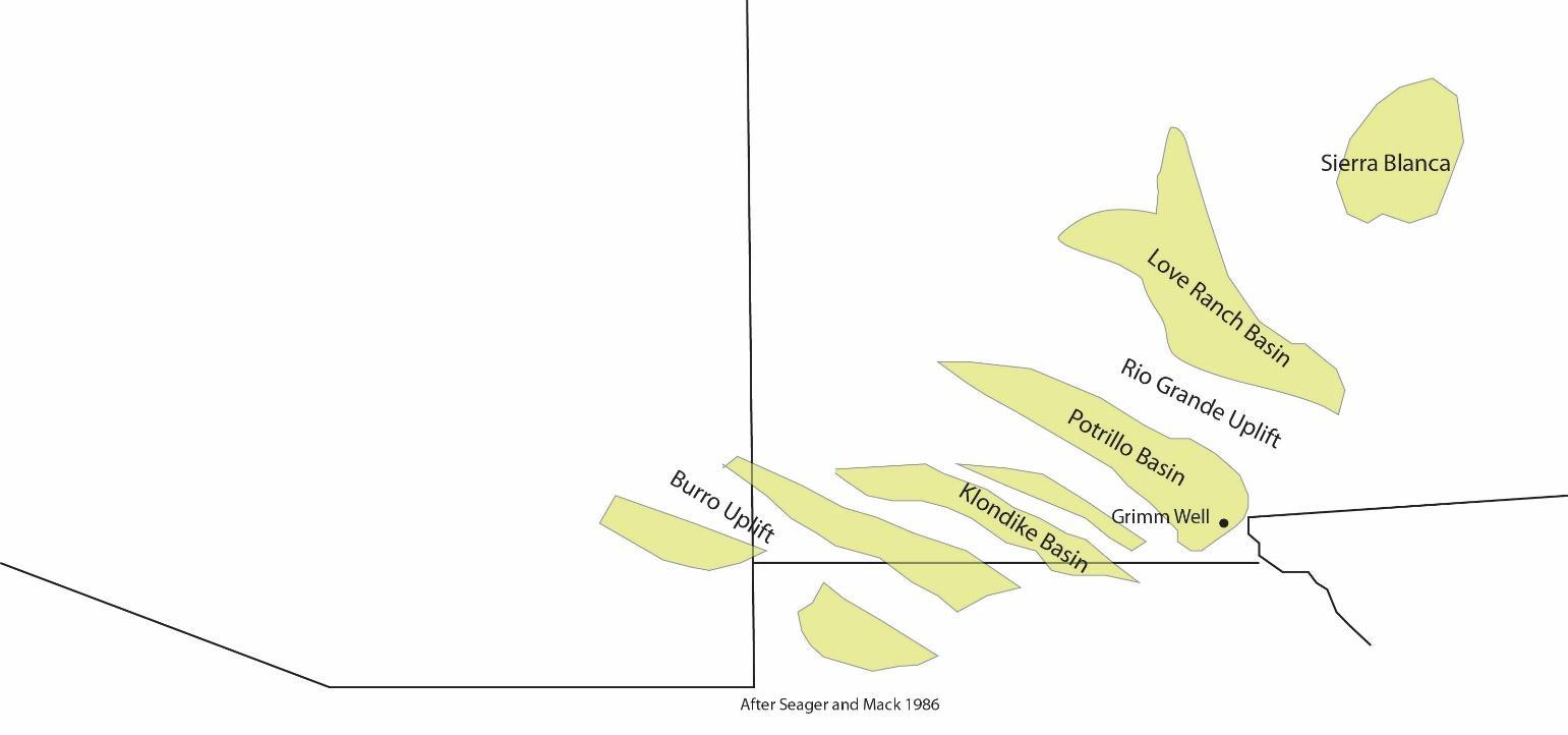
88
Figure 7-1 Laramide Basins of the El Paso Area. (Geology derived from De los Santos, 2018).
The Love Ranch grades upward into the volcanic clast conglomerates of the Palm Park and Rubio Peak Formations (Seager and Mack, 1986). The volcanos, volcanic intrusions and the sediments derived from them are an important part of the late Eocene in the El Paso area, and are different from Laramide features farther north. In the El Paso area Eocene aged igneous intrusions are distinctive and important features (See Map). The most prominent Eocene features in El Paso are shallow intrusions that form laccoliths and sills; the softer sediments have eroded around them and they form hills and small mountains. The tallest is Sierra Cristo Rey, which is 48 million years old, the Campus Andesite that the UTEP campus sits on is 47 Million years old, other similar hills include the Three Sisters Hills, and the Thunderbird and Coronado Intrusions on the Western side of the Franklin Mountains (Hoover et al., 1988). (See Map). Additionally, 50-million-year-old andesite dikes were emplaced in the Sierra de Juarez.
During Eocene time, El Paso was far removed from the western subduction zone produced by the Farallon Plate/North American Plate collision and the Andean model for our andesites seems inappropriate. Geophysical studies have suggested that an answer to this apparent paradox is that a segment of the Farallon Plate was subducted at a lower -thannormal angle (Figure 7-2) so that the subducted slab did not get deep enough to get hot enough to melt until it was much further "inland" than normal. Most researchers agree with a tectonic model where Laramide deformation and volcanism were due to this “flat slab” subduction from 75 million years ago to-35 million years ago (Coney and Reynolds, 1977)

89
Figure 7-2 (a) Normal “Andes” type subduction. (b) low-angle subduction similar to the subduction of the Farallon plate (figure from opengeology.org)
The Great Ignimbrite Flare Up
To the east of El Paso, a new phase of igneous activity commenced about 35 million years ago with igneous intrusions of silica-rich magmas that produced the intrusive peak called Cerro Alto in the northern Hueco Mountains and the mass of igneous rock forming Hueco Tanks. Farther east syenites and phonolites formed intrusions and volcanoes on the Diablo Plateau in the Cornudas area. Syenites are rocks with lots of Aluminum, and Sodium, but with less silica, so that unlike granites, little quartz crystalizes (Nutt and O’Neill, 1998) At about the same time, igneous activity began to occur in southern New Mexico (Figure 7-3). The first eruptions in New Mexico were in the Organ Mountains near Las Cruces, and volcanism gradually migrated to the northeast (McIntosh et al., 1992) The eruptions in Texas and southern New Mexico mark the beginning of the “Great Ignimbrite Flare Up” during which great volumes of volcanic eruptions, most commonly volcanic ash, blanketed the western US and Mexico between 36 and 18 million years ago (Best et al., 2013).
The emplacement of large-scale ignimbrites in the southwestern U.S. during and following the Laramide orogeny has been attributed to the flow of hot asthenosphere into the upper mantle as the Farallon plate subsided from beneath North America (McMillan et al., 2000)
Where not broken and partially buried by later extension of the Rio Grande rift, these volcanics formed mountains as they piled up on the surface. Many of the major features of the El Paso region were formed at this time. The largest is the great mountain range of Mexico, the Sierra Madre Occidental (Figure 7-3). The Gila Mountains and Black Range, Sierra Blanca, the San Juan Mountains of Colorado, the Davis Mountains, and most of the Mountains of the Big Bend all are eroded volcanic complexes formed during the ignimbrite flareup (Figure 7-3).
Unlike the older Eocene igneous rocks, the rocks of these ranges were more mixed compositionally and include significant amounts of volcanic ashes and lava flows. Most of the eruptions were huge explosive eruptions forming calderas. Calderas are typically roughly circular in map view with pronounced central depression surrounded by a high rim, giving them a cross-section resembling a large cauldron or soup bowl, thus the name. Calderas form through giant eruptions, where a large magma body gets close to the surface. Pressure builds within the magma, which eventually explodes along ring shaped fractures, expelling cubic kilometers of ash. This leaves a void beneath the surface and the lid of the caldera falls into the magma chamber. This creates the caldera at the surface, which is usually largely filled with thick ash deposits. Ash from the eruptions is spread widely across the landscape. To give one example, much more recent ash from Yellowstone in Wyoming can be found in El Paso. The ashes were interbedded with sediments in Eocene and Oligocene basins across the region, allowing us to date sediments and fossils.
90
A four-phase history is typical of calderas (Figure 7-4). In the first stage, plutonic magmas are emplaced into the near surface, usually doming the host rocks upward over the main magma body. The second stage is the main eruptive phase, magma breaks through the dome and great volumes of volcanic ash are released, eventually leading to collapse of the central “lid” along a series of normal faults that form a more or less complete ring separating the collapsed floor from the high-standing rim. Phase three is the resurgent phase during which new magmas move into the main chamber and build a resurgent dome on the caldera floor. The resurgent dome is not a volcanic eruption, but the doming of the caldera floor as new magma flows in from below. In phase four, magma invades the ring fault system and forms ring dikes. Some of this magma may reach the surface to form lava flows that spread

91
Figure 7-3 – Areas covered with deposits of the Eocene-Oligocene Great ignimbrite flare up (orange). From (Best et al., 2013). Added under Geological Society of America Fair Use Provision
into the caldera as moat deposits between the ring dikes and the resurgent dome. Other magma may produce small volcanos along the ring fracture.

Early Rift Extension
Early Rio Grande extensional faulting began at approximately the same time as the Great Ignimbrite Flare up sediments. The earliest rift basins have been dissected and replaced with younger basins, however the sediments that fill them are exposed in isolated outcrops. The oldest of these is the Bell Top Formation which was deposited in a rift containing 35 million year old ashes (Mack et al., 1994). An unconformity separates the Palm Park from the Bell Top Formation. Bell Top rocks consist of 2,000 feet (850 m) of Oligocene volcanoclastic sediments and tuff beds. Flow-banded rhyolite and basaltic andesite sills and dikes occur as well. The Bell Top was deposited in a half-graben that formed in the area between Las Cruces and Truth or Consequences (Mack et al., 1994).
Uvas basaltic andesite covers the Bell Top. It consists of 400 feet (120 m) of basaltic andesite flows and cinder beds as well as a variety of volcanoclastic sediments. One of the andesite flows has a radiometric ages of 25 million years, as well as a doubtful age of 31
92
Figure 7-4 – Caldera formation (from National Park Service)
million years (Clemons and Seager, 1973). This puts the Uvas in the Late Oligocene and Miocene, during the latter part of the Great Ignimbrite Flare up.
The Rio Grande Rift
Most of the El Paso Landscape is shaped by the Rio Grande rift. The Rio Grande rift is one of the most dramatic features in North America, and is also one of the youngest. The continent has been stretched in the El Paso area, and this has resulted in a landscape of basins separated by tilted fault-block mountains. The Rio Grande River flowed down the rift, filling basins with sediment, finishing the classic El Paso Landscape of steep-sided mountains, surrounded by flat desert surfaces that overlie deep basins. Most of the earlier features we have discussed are evident as layers and patches within the mountain ranges.
The Rio Grande rift is a north-south-trending alignment of extensional basins and uplifts extending from Colorado to El Paso. As discussed above, rifting began in the Oligocene (Mack et al., 1994). However, this early phase of extension in the rift does not seem to have resulted in large faults and mountain ranges. The main phase of rifting that created the Franklins, Organs, Huecos, Potrillos and Sierra de Juarez seems to have begun about 25 million years ago, during the Miocene (Ricketts et al., 2016) This dating comes from thermochronologic data, which shows when rocks in the rift-flank mountains were uplifted to near the surface and cooled (Ricketts et al., 2016). In Colorado and northern New Mexico, the rift forms a narrow trough between the Colorado Plateau and Southern Rocky Mountains. In southern New Mexico, south of Socorro, New Mexico, it splits into several parallel basins separated by narrow mountain ranges. In Trans-Pecos Texas, rift extension began about 31 to 28 Ma based on the orientations of dikes and fault movement data (Henry et al., 1991)
This main phase of rifting raised mountains up and dropped the basins along faults. These are big faults. The offset of equivalent strata on the East Franklins fault is about 15,000 ft (5 km). Extensional faulting, like the Rio Grande rift creates, three main features. Tilted blocks, horsts and grabens (Figure 7-5) Tilted fault blocks form where the earth is stretched, instead of having faults dipping in two directions the faults all dip the same direction ( Figure 7-6). As extension continues the faults become lower angle and the blocks in between become more and more tilted.

93
Figure 7-5 Horsts and grabens formed by normal faults in areas undergoing extension such as the Rio Grande rift. Image public domain from USGS.
The Franklins are a tilted horst block, which is a combination of the two styles above (Figure 7-7). A fault with about 2,000 ft. (610 m) of displacement is buried along the front of the Hueco Mountains, separating the Hueco graben from the Hueco Mountains. The Huecos are only somewhat higher than the Diablo Plateau onto which they merge. The Hueco Mountains are really just the uptilted edge of the plateau, and have been tilted by the rift extension. The Diablo Plateau has not been extended and is basically flat, and has been since the Permian, when the Ancestral Rockies orogeny finished. West of the bounding fault, the Hueco basin steps down across a series of smaller faults (Figure 7-7). It reaches its deepest along the east side of the Franklins, where the East Franklins fault separates the Hueco Basin from the Franklin Mountains.
The Franklin Mountains are a tilted horst block; beds in the Franklins dip at least 40 degrees to the west and, in the north part of the range, can be almost vertical. There are several older faults that angle from southeast to northwest across the range, or make semicircular outcrops. Typically these older faults dip at 45 degrees or less. The most prominent of these are the McKelligon Canyon and Fusselman Canyon faults, which follow the

94
Figure 7-6 Tilted fault blocks, showing the effects of progressive extension. Drawing from Wikimedia commons under Creative Commons share alike from Aturn4000.
bottoms of the canyons they are named for. Enhanced erosion along these faults probably accounts for the locations of these canyons.
On the west side of the Franklins, an enigmatic of set of faults follow the edge of the range. There is almost certainly Late Tertiary and Quaternary movement on these faults as Pliocene gravels discussed in the next chapter are faulted against the bedrock of the Franklins. There is also a reverse or thrust fault that follows the same trend. Folded and faulted Cretaceous sediments can be found as far north as Coronado Country Club, in a narrow band, sandwiched between the Franklins and hills made of Permian strata. This fault, stopped moving about 5 million years ago and a new active fault formed running along Interstate 10. This fault (Figure 7-7) separates the deep Mesilla Basin from a shelf with uplifted rift sediments that have been eroded to form terraces and mesas. Small hills across west El Paso expose andesites intruding Cretaceous shales and limestones.
Rift Sediments
The subsiding grabens and half grabens around El Paso, were filled with sediments. Sediments of the Rio Grande rift are known as the Santa Fe Group, and are mostly buried beneath the basins, where they have only been encountered in wells. However, north of El Paso, in the rift basins near Hatch and Truth or Consequences, the shifting of fault movement has brought some of the older sediments near to the surface. These sediments have a variety of names in different parts of the rift, but in general they can be grouped into Lower Santa Fe Group sediments, of mostly Miocene age, Middle Santa Fe Group sediments of Late Miocene age, and Upper Santa Fe group sediments of Pliocene to recent ages.
The exposed Santa Fe Group sediments in southern New Mexico, are divided into three formations: the basal Hayner Ranch Formation, the Rincon Valley Formation, and the upper Camp Rice Formation. Conglomerates of red to orange pebbles and cobbles, conglomeratic sandstones, sandstone, and minor amounts of siltstone comprise the Hayner Ranch. The thickness of the unit is about 2,000 feet (600 m) and the unit is thought to be Middle Miocene in age. The Rincon Valley Formation is 1,300 feet (400 m) thick and is composed of fine-grained clastic sediments intruded by a 9-million-year-old basalt sequence. In places gypsiferous claystone is present. Overall, well data shows most of the rift sediments to reflect deposition in flat basins surrounded by steep mountains, with coarse gravels next to the mountains and playa mudstones in the centers.
The uppermost sediments in the Santa Fe group crop out along the Rio Grande valley and along faults on the east side of the Franklin mountains. The mostly older sediments reflect deposition that is not greatly influenced by the Rio Grande and are called the Fort Hancock Formation. Fort Hancock sediments are conspicuous around El Paso. They were defined from outcrops near Fort Hancock Texas, about 60 miles (96 km) southeast of El Paso and are exposed along the Rio Grande and its flanking arroyos between the southeast end of the Hueco Bolson and El Paso. To the west, they form bluffs along the edge of the West Mesa from the border, through Santa Teresa to La Union; they are exposed in highway cuts along I10; the bluffs directly north of El Paso High School are Fort Hancock beds; and roads cuts along Alabama and Magnetic Streets expose Fort Hancock beds as well. As much as 400 feet (120 m) of Fort Hancock strata crop out locally. Correlation with the equivalent upper Santa Fe group sediments is difficult due to the complex changes across the basins. However, the Fort Hancock may reach as much as 4,300 feet thick (1,310 m) in the Hueco Bolson (Hawley et al., 2009)
Clays in the Fort Hancock create building problems because they swell and shrink as their water content changes. Generally, Fort Hancock beds are buff to brown silts, clays, and sands deposited in a series of playa lakes and their bordering alluvial fans. Playa lakes are
95
intermittent features, water-filled during wet periods and dry mud flats during dry ones. Wetting and drying typically causes clayey sediments to shrink and swell, obliterating the bedding. The conglomerates are typically coarse and contain clasts derived from the adjacent mountains.

A variety of fossils occur in Fort Hancock sediments, including aquatic beasts such as beaver and turtles, and terrestrial animals such as horses, camels, rabbits, and mammoths. These fossils are part of a distinctive vertebrate assemblage, the Blancan Assemblage, of western North America. The Blancan broadly corresponds to the middle and late Pliocene (from 4.75 to 1.8 million years ago) and marks the time when North America and South America were connected by the Isthmus of Panama, leading to the Great American Interchange of animals that had developed in isolation up till now.
The Rio Grande
The top of the Fort Hancock formation is marked by the appearance of sediments of the Rio Grande. The story of the Rio Grande is the story of the Rio Grande rift. Opening of the Rift created a trough that extended from central Colorado to El Paso. Originally the rifting created a series of basins that were isolated from each other. Because there was more precipitation in the high mountains of the San Juan and other ranges in Colorado, more sediment was eroded, and the basins in the north of the rift filled first. The mountains and basins of the rift that we see today are young. The first sediments date to 10-12 million years ago (Seager et al., 1984; Langford et al., 1999) The proto Rio Grande first filled the San Luis Basin by about 9 million years ago and appeared in Albuquerque by about 7 million years ago By 5 million years ago, the Rio Grande first appeared in the El Paso Region (Mack et al., 1998)
96
Figure 7-7 Cross Section through El Paso from the eastern Mesilla Basin to the Hueco Mountains. Figure is not to scale. Topography is exaggerated 10:1. Unit thicknesses and dips are approximate. Thrust and reverse faults are probably Laramide. Normal faults are Neogene Rio Grande rift.
Some of the oldest Rio Grande channel sandstones are found on the west side of the Franklin Mountains, where they have been faulted up along with the Franklin Mountains and underlie the prominent Mesas along Mesa St (Figure 7-7). There are no specific dates for these uplifted terraces, however the amount of uplift with the Franklins suggests they are 4-5 Million years old.
After its initial appearance, the Rio shifted from basin to basin in the El Paso area (Figure 7-8) (Hawley et al., 2009). About 3.5 million years ago, the Rio Grande had filled the Mesilla Basin enough that it was able to flow through the Fillmore Pass between the Franklin and Organ Mountains (Figure 7-8). Eventually it created a great fan that separated the Hueco and Tularosa Basins. Before this time, there was no divide separating the two basins. After this, the Rio flowed episodically into the southeastern Hueco basin and the Tularosa basin creating lakes that lasted until the river shifted again. Throughout this time, the Hueco basin in East El Paso was a playa lake that episodically filled. Deposits of the Rio Grande channels are restricted to a zone between Fort Bliss and the Franklins.
By about 3 million years ago the Rio Grande was episodically flowing across La Mesa, west of El Paso, all the way to Deming and the Mimbres River Valley. However, continued subsidence of the Mesilla Basin and uplift of the Potrillo and Hueco Mountains lifted these

97
Figure 7-8. Terminal basins of the Rio Grande with the ranges of times they were first occupied. Modified from (Hawley et al., 2009)
sediments up and blocked off access to the west of the Potrillo Mountains. Soon after this, about 2 million years ago, uplift of the Franklins and Organs blocked access through the Fillmore Pass (Figure 7-8). After this time, the Rio was restricted to the Mesilla basin until it reached the pass near downtown El Paso. Therefore the Mesilla Basin contains a zone of Rio Grande sands as thick as 1000 ft. (300 m).
Deposition of the Camp Rice formation from Rio Grande sands continued into the Pleistocene. Camp Rice sediments consist of two interfingering lithofacies. Along the flanks of highlands, piedmont gravels deposited from alluvial fans. The others are fluvial channel sandstones and associated floodplain rocks of the Rio Grande. Most of the pebbles in the channel sands are “exotic” and were eroded and transported into this area from sources well upstream in the ancestral Rio Grande drainage system.
By about 2 million years ago, at the end of the Neogene period, the El Paso landscape was starting to look similar to what we see today. The Rio Grande rift had reshaped the region, the Franklin, Organ, Hueco, Potrillo Mountains and the Sierra de Juarez had assumed much of their present shape. The Hueco and Mesilla basins had largely been filled and the Rio Grande flowed across the complex of floodplains and lake basins. The climate and wildlife were very different, with mammoths and mastodons, sloths and camels and horses roaming what was probably a much better vegetated landscape. However there was one more major act still to come, the Quaternary.
Crazy Cat "Mountain" is a landslide formed during the Quaternary. It involved Ordovician Aleman and Cutter formations and Silurian Fusselman dolomite. Rocks of the slide were shattered as they slid, suggesting that it was a catastrophic event. Subsequently, ground water percolating through the mass dissolved and re-precipitated some of the calcium carbonate to re-cement the slide. The slide took place as the Rio Grande flowed along the western side of the Franklin Mountains, probably undercutting the layers of rock, destabilizing the mountainside. The slide front covers floodplain sediments along Piedmont Street while its eastern side overlies channel sands and gravels containing exotic clasts from the north
98

99
Figure 7-9 is a physiographic map of the El Paso area.
CHAPTER 8 - FIRE AND LAKES – El PASO IN THE PLEISTOCENE
Volcanos
The Rio Grande rift not only created the mountains and basins that we see in the El Paso area, it also stretched the earth’s crust and lithosphere, allowing hot mantle material to flow up to more shallow levels. This reduced pressure allowed some of mantle to melt and the faults in the crust allowed the magma to reach the surface, creating volcanos. There were volcanic eruptions throughout the Tertiary, but the most recent one began in the desert west of El Paso near the beginning of the Pleistocene. Figure 8-1 shows the main volcanos west of El Paso. Most of these fall in three north south linear sets, probably because they were fed from faults. From east to west, these are the 1) Black Mountain-Santo Tomas area, the 2) Aden-Afton area, and the 3) West Potrillo field (Figure 8-1). The East Potrillo hills are a tilted fault block range of Permian and Cretaceous rocks, while Mt. Riley is an intrusive pluton of rhyodacite of Eocene age. The West Potrillo field, covering 300 square miles (777 km2), is the largest.
The oldest features are cinder cones in the Potrillo volcanic field that may be as old as 2 million years and are mostly buried under younger volcanos. More recent features form distinct cones on the landscape. There are two main types of features, cinder cones and maar volcanos. The cinder cones are small steep sided cones with small craters in the top (Figure 8-2). Cinder cones usually form from basaltic magmas as a fountain of magma sprays from the vent. The magma breaks into chunks which inflate like popcorn, as they are full of gasses when they erupt. The larger pieces form volcanic bombs and the smaller form cinders (https://en.wikipedia.org/wiki/Cinder). Cinders are typically 1 to 10 cm across and are very light due to the holes, called vesicles within them. Most El Pasoans are familiar with the black, brown and red cinders used as ground cover in yards and called “lava rock”. Most of these are mined from cinder cones in the region.
100


101
Figure 8-1. Google earth image overlain with the locations of the prominent volcanic features west of El Paso (image from Landsat/Copernicus).
Figure 8-2. Google earth image looking west of two cinder cones in the northern part of the Potrillo volcanic field, looking west. The nearer cone has a crater with a small dry pond in it. The farther has a breached crater, with a lava flow coming out the left side. (image Google Earth from Landsat/Copernicus).
The cinder cones are usually rounded with steep slopes. Many of the cinder cones have been breached. This means that as the cone grew by adding new layers of ash, lava rose inside the cone. Also, as the eruption proceeded, the gas in the lava was released, and instead of exploding to create a fountain, the lava began to flow. It rose in the cone and the pressure of the lava pushed the cinders on one side away, and lava flowed out of the side of the cone.
The nearest cinder cones to El Paso are. Black Mountain, Little Black Mountain, San Miguel and Santo Tomas, which lie in a chain along the West Mesa. Black Mountain is the largest and southernmost, Little Black Mountain lies next along the Black Mountain fault, and is the smallest. The San Miguel center is next and the field ends at the Santo Tomas eruptive center. Little Black Mountain and the San Miguel center appear to have erupted only once, building small cinder cone systems, some 250 feet (76 m) in diameter and 15 - 20 feet (4.5-6 m) high. Black Mountain and Santo Tomas erupted repeatedly and built large cinder cones. Black Mountain stands about 2,000 feet (600 m) in diameter and stands about 300 feet (90 m) above the La Mesa surface. Santo Tomas is smaller. Lavas of the Black Mountain-Santo Tomas field are olivine-rich basalts. Quarrying for light-weight aggregate has exposed the internal structure of Black Mountain. It consists of layers of volcaniclastic rocks including ash and cinder (clasts less than 4 mm in diameter) beds, beds of lapilli (rounded clasts 4-32 mm in diameter), and volcanic bombs. Bombs, by definition, exceed 32 mm in diameter and some in Black Mountain are 2 m in diameter.
Lava flows spread outward from the cones through lateral vents on the flanks. Near Stahmann Farm, one of the flows from Santo Tomas flows down the valley border slope. Along its eastern edge, erosion by the Rio Grande that produced the Kern Place Terrace has undercut the lava flow. This bit of geomorphic evidence indicates that the down cutting took place after the flow. Radiometric dates on the Santo Tomas flows are 80,000 to 100,000 years old (Williams, 1999).
The next volcanos to the west are in the Aden-Afton area. These volcanos are aligned with two normal faults (see Chapter 3), the Fitzgerald Fault on the east and the Robledo Fault on the west (Figure 8-1). The Afton Basalts extruded in three separate flow phases (AF-1, AF-2, and AF-3) along the Fitzgerald fault (Hoffer, 1976) (Figure 8-3). AF-1 was emplaced across what later became Hunt's Hole and Kilbourne Hole but its source has not been located. Northeast along the fault, AF-1 flows are overlain by AF-2 flows in the vicinity of Gardiner Cone, a cinder cone in the center of the field. There AF-3 over- lies AF-2 in a small area around the cone which was most likely the source of the AF-3 flow. The Afton flows are also olivine-rich basalts but are similar in age to the Black Mountain-Santo Tomas basalts, having isotopic and soil dates of 110,000 to 88,000 thousand years (Williams, 1999). In the northwest portion of the field, two (perhaps three) younger flows are present. A-1 is overlain by A-2 near Aden Crater and along the Aden Fault near small collapse craters.
Aden Crater is the youngest and most obvious feature of the Aden-Afton Field. Helium exposure dates and isotopic dating suggest an age of 45,000 for the older flow and 21,000 years for the younger (Williams, 1999). The cone is a circular, steep-sided pile of volcaniclastic basalt that rises 200 feet (60 m) above the La Mesa surface. It is 1,350 feet (410 m) in diameter. Inside the rim, a flat floor of basalt covers most of the area, although a 300 foot (91 m) diameter collapse crater occupies the southeastern quadrant (Figure 8-4). Development of Aden Cone began with an eruption from a central vent around which lava accumulated. Explosive venting followed, building up a rampart of spatter, cinders, lapilli, and bombs (Hoffer, 1976). Once the rampart (exterior walls) began to grow, lava pooled inside producing a lava lake. Some of the lava spilled over the rampart and some oozed through it to flow off the flanks building lava tubes, lava ridges, and herraduras (horseshoe shaped lava
102
ridges). As the lava lake cooled and shrank, tension cracks developed around the margin and small spatter cones arose along this fissure system. While the lake was cooling, the rampart was breached along the eastern edge and some of the lava drained out, undermining the solid lava surface to produce the collapse structure. Volcanic gases escaping during this phase forced their way upward through the rampart and burst out, forming a fumarole. In the 1920s, the fossilized remains of a ground sloth (Nothrotherium shastense) were recovered from the bottom of the fumarole. Carbon14 dating of the associated bat guano indicates that the sloth died about 11,000 years ago. The specimen is the most complete set of skeletal remains yet recovered from a single sloth (https://www.utep.edu/leb/pleistnm/sites/adenfumerole.htm).
The uplifted western side of the Robledo Fault marks the eastern edge of the West Potrillo Field, a tilted horst block whose western boundary is unidentified (Figure 8-1). The West Potrillo Field (Figure 8-1) covers almost 300 square miles (770 square km). More than 150 individual cinder cone volcanoes have been identified within the field and many have extensive lava flow systems around them. Radiometric ages and helium exposure dates range have been obtained on basalts of the West Potrillo Field, these range in age from 850 to 200,000 years old (Williams, 1999)
Maar Volcanos
The other dramatic features of the Potrillo volcanic Field are maar craters, There are five well exposed craters surrounded by volcanic ash (Figure 8-1) These are Kilbourne Hole, Hunt's Hole, Potrillo Maar (called Cerro el Volcán in Mexico), Malpais Maar, and Mt .Riley Maar. A maar is a broad volcanic crater formed by shallow explosive eruptions. The explosions are usually caused by the steam explosion that happens when magma gets near the groundwater table and the water boils. This unusual volcanic event is not unlike a pressure cooker exploding from the immense pressure building from the boiling water inside.
Kilbourne Hole (Figures 8-1, 8-4) is the largest maar, approximately 1.5 miles (2.4 km) in diameter. In the lower parts of the crater walls, Camp Rice Formation sediments are exposed on the inner slopes of the crater. Camp Rice sandstones contain exotic clasts showing the Rio Grande flowed through this area. The Camp Rice mudstones are capped by a thick calcic soil showing the land was stable. This type of soil typically requires at least 300,000 years to form, so for possibly a million years this area was probably a grass and treecovered plain. The Camp Rice and its soil is covered by 12 feet (3.7 m) of olivine-rich basalt that formed a tight cap over the sediments. This AF-1 basalt is dated to about 120,000 years old.
The eruption of Kilbourne Hole occurred about 30,000 years ago as estimated by Helium exposure dates (Williams, 1999). The volcano created the crater, and the debris formed a gentle cone of ash around it. The ashes reach up to 160 feet (48 m) thick. The lowest unit is a cross-bedded, hard medium gray ash, containing large cross-beds. Such explosive blasts usually have two components - a vertical blast and a lateral blast. In the vertical blast, shattered caprock was flung upward and outward while the lateral blast (or the base surge) of gas and dust spread sideways along the ground surface. The ejecta blanket from Kilbourne Hole covers an area 5 miles (8 km) in diameter. That of Hunt's Hole is about 2.5 miles (4 km) in diameter.
103
is the youngest. The Gardener Volcanos are three craters within a composite cinder cone. Aden Volcano is a large crater within a breached cinder cone. AD-1 is the older Aden flow and AD2 is the youngest, and the youngest volcanic feature in this map. (satellite image Google Earth from Landsat/Copernicus).
These beds are actually giant climbing ripples and the foresets dip away from the crater in all directions showing they were created by explosions from the volcano. This layer is called a base surge deposit. Base surges are the sediments laid down at the base of a swiftly

104
Figure 8-3. Map of the lava flows and Maar Volcanos in the Kilbourne-Aden-Afton area. The maar volcanos creating Kilbourne and Hunts holes erupted through the oldest Afton flow (AF-1), which shows as the black rim around the craters. AF-1 is the oldest Afton Flow, AF-2 is the second, and AF-3
moving ash flow, where sediment settles out. The base surge is created by the air and ash squeezed from beneath the ash cloud. Close inspection of the base surge layers shows that particles range from coarse sand to about a centimeter. Most of them are a couple of millimeters across and are therefore in the lapilli size range. Fine grained volcanic ejecta is called ash, centimeter to 10 cm sizes are called cinders, and the largest fragments are called volcanic bombs. Volcanic bombs can be found within the base surge deposits and deform them, showing the base surge layers were soft and muddy after deposition. Erosion surfaces separate repeated layers of base surge ripples, showing that the base surge formed from a series of explosions from the crater. Close inspection of the base surge lapilli shows they are actually composed of balls of fine grained volcanic ash, sort of mini-mud-balls. You can imagine Kilbourne hole exploding every few hours, erupting clouds of steamy ash in all directions.
The uppermost layer at most of the Maar volcanos, including Kilbourne Hole is a poorly sorted, poorly bedded basaltic silt, sand and lapilli with small angular blocks of basalt. This unit formed though the final explosions from the craters, which must have been more vertical. As the particles settled, the wind blew them to the northeast, where they form a blanket extending from the volcano. This settling from the air creates a deposit called an airfall tuff The thickest deposit of this airfall tuff is found along the crater rim along the east and north sides (Figures 8-4, 8-5). The bedded tuff is thickest on the eastern flanks of the crater and thinnest on the southwestern side. Hunt's Hole exhibits the same features, on a smaller scale. However, it is younger, and is approximately 20,000 years old (Williams, 1999).

105
Figure 8-4. Map of Kilbourne Hole showing the distribution of the air-fall tuff and base surge deposits. The dark rim around the crater is the AF-1 flow from the Afton volcanic center. (image Google Earth from Landsat/Copernicus).
Recent studies have indicated that the crater is filled with debris from the explosions to a depth of 1 km with breccia and ash from the eruption (Maksim, 2016) Beneath this, three dikes formed intrusions beneath the crater. These dikes encountered groundwater in the Neogene sediments beneath the crater, and caused repeated eruptions of ash and superheated steam (Maksim, 2016). Pressure built below the older lava flow caprock until the bubble burst through the AF-1 caprock in an explosive eruption of magma gas or steam or both. No doubt this would have been one of the largest natural explosions in El Paso’s history.

106
Figure 8-5. Photo of the east wall of Kilbourne Hole showing the stratigraphy. The light gray and pinkish layers in the bottom are Camp Rice formation, with Rio Grande channel sandstones. The dark black in the right foreground and the thin layer on the left side of the crater wall. Eroded basalt boulders cover the slope on the left side making it look black. On the right side, a grayish white layer at the top of the pink is a calcic soil, and this is overlain by a darker pink baked horizon, that was cooked by the AF-1 flow. The base surge deposits are the medium gray layer overlying the basalt. The air fall tuff is only found on the northeast and east sides of the crater.
Chapter 9 - EARTHQUAKES, FAULTS AND THE SHAPING OF THE EL PASO LANDSCAPE
It often surprises people that earthquakes occur in the El Paso region. They certainly do not happen as often as in California or Alaska, but on average an earthquake is felt (at least by some) in the El Paso area once every 10 years. Earthquakes in the El Paso region (Figures 9-1 and 9-2) can occur for a variety of reasons. The most common source of earthquakes in our region is the ongoing tectonic activity associated with the Rio Grande rift. As the crust continues to be pulled apart by tectonic forces, we have earthquakes. A second cause of earthquakes is the movement of magma and hot fluids in the subsurface. These type of earthquakes are common in areas of recent volcanic activity. One of the more active regions over the past 100 years is located south of Socorro, New Mexico (Figure 9-1) where geophysicists have imaged a magma body in the subsurface at depths of ~20 km. Movements of magma or fluids often produce earthquake “swarms” – many small earthquakes similar in size. The most dramatic of these in the Socorro area occurred in 1906 and included two to three earthquakes of magnitude 5.8-6.2. The third cause of earthquakes is related to human activities including crustal loading produced by water reservoirs, oil and gas production, mining and injection of fluids into the ground. At least some of the earthquakes in the Permian Basin of west Texas and southern New Mexico could be related to human activity but many are also related to tectonic activity and it is often difficult to pinpoint which of these is the ultimate cause.
Whatever the causes of the earthquakes, most are too small to be felt (less than about magnitude 2.5), but can be recorded by sensitive detectors of ground motion (seismometers) that amplify ground motion hundreds of thousands of times. Figure 9-3 shows the location of seismometers as of fall 2021 in the El Paso region. Most seismometers relay ground motion information via the internet to a variety of earthquake centers where the records of ground motion (seismograms) are stored digitally on computers. Gone are the days of ink pens shaking wildly over drums covered with paper during earthquakes, as commonly seen in disaster movies. A few pen and ink seismographs (machines that display ground motion) still exist in museums or special displays – much more dramatic than an image on a computer screen.
Digital recording of earthquakes on computers allows scientists to rapidly locate and determine the magnitudes of the events. Initial locations and magnitudes are often automatically determined by computer algorithms and then checked by humans. In places like California or southern Mexico where large earthquakes are frequent, computer algorithms will broadcast warning messages via the internet and cell phones if a large earthquake has been detected, allowing people 10 to 30 seconds to prepare for the oncoming earthquake. This is enough time for power companies to turn off electricity or gas and for people to seek shelter (under tables or desks) or move away from dangerous areas (such as shelves with heavy objects).
Significant felt earthquakes of the region over the past 100 years are shown in Figure 9-2. These earthquakes have magnitudes greater than 5. Recall that magnitude is a logarithmic measurement of the amplitude of ground motion produced by an earthquake. This means a magnitude 5 produces 10 times the ground motion amplitude of a magnitude 4 earthquake and 100 times the ground motion amplitude of a magnitude 3 earthquake. Another factor that determines the severity of shaking besides the magnitude is the soil and rock conditions at a specific site. Loose soil and especially loose, wet soil shakes more than a site near or on bedrock. Thus the 2020 Mentone, Texas earthquake (magnitude 5.0) was more
107
strongly felt in El Paso’s Upper and Lower Valley where soil is loose and the water table is high than in the regions of the city located above the river valley. The measurement of shaking and damage is called “intensity” and is usually denoted by Roman numerals so that it is not confused with magnitude. Figure 9-4 shows the intensity pattern for the Mentone earthquake based on online surveys that “citizen scientists” filled out at the internet site “Did you feel it?”
(https://earthquake.usgs.gov/data/dyfi/) operated by the U.S. Geological Survey.
The largest earthquake in Texas (magnitude ~ 6.3) occurred near Valentine, Texas in 1931 (Figure 9-2). It was felt strongly in the El Paso region, causing some people to run outside their houses and chickens to fly wildly around barnyards. Minor damage was experienced in the sparsely populated Valentine region. Because rocks in east Texas are cooler and transmit earthquake energy better than the warmer, broken up rocks of west Texas and southern New Mexico, the Valentine earthquake was felt as far away as San Antonio and Dallas. The second largest earthquake in the west Texas region (magnitude ~ 5.8) occurred in 1995 between the towns of Alpine and Marathon. Because it caused more damage in Alpine, it is often called the “Alpine earthquake”. Fortunately, earthquakes recorded within El Paso county (Figure 9-5) have only been felt (magnitude 2 to 3 range) by people living very close to them. However, as you will discover later in this chapter, our region has numerous active faults that are capable of producing magnitude 7+ earthquakes and local emergency responders now include earthquakes (along with fires, floods, chemical spills, airplane crashes, etc.) in disaster preparedness and response planning.
108
Socorro Swarm

109

110
Figure 9-2 – Earthquakes of Magnitude > 5.0 occurring in the El Paso region. Figure created by D. Doser (2021).

111
https://earthquake.usgs.gov/earthquakes/eventpage/us70008ggn/dyfi/intensity

112 website:
Faults
By about 2 million years ago, the Rio Grande had filled most of the basins in the El Paso area and created a fluvial plain, a gently sloping plain created by flooding of the Rio Grande. The Rio Grande shifted from basin to basin. As we have seen, volcanos erupted onto this plain. However, the Rio Grande rift is still active, and once the river had leveled the topography, the rift faulting began to lift the mountains and drop the basins (Figure 7-7). As each basin was isolated by uplift of the adjacent mountains, the landscape created by the Rio Grande was preserved as a relict alluvial plain, a landscape created by a river that no longer flowed there. Much of the basin floors around El Paso have not been greatly changed during the last 500,000 to 2 million years.
However, the continued rifting continued to stretch the basins, and faults formed within them. Many of these faults are evident in the basin floors today and can be seen on satellite images (Figure 9-6). This subtly reshaped the basin floor into a series of flat steps separated by slopes that trace eroded fault scarps. Drifting sand and erosion have

113
covered and reshaped these features so they are often difficult to recognize unless you are looking for them. However, from the air, they are obvious due to the mesquite and grass that preferentially grow along them.
These surface faults have dropped the Hueco Basin so that it is lower than the Mesilla Basin. Near Las Cruces, the Robledo Fault has dropped the Lower La Mesa surface to about 100 m below the Upper La Mesa Surface. Originally these were contiguous, forming one flat plain.
The Pleistocene Pluvial lakes. Deformation of the basins along the Quaternary faults created low areas where the basins subsided the most. Unlike the relict plains around them, the lakes in the bottoms of the basins continued to accumulate sediments to the present. As long as the Rio Grande continued to flow into them, these lakes were semi-permanent, but when the Rio connected to the Gulf of Mexico as discussed below, the lakes became controlled by the local cli mate.
114
Figure 9-6. Fault map of the El Paso Area. The red lines are faults that are known to have been active in the Quaternary. Not all of the faults in Mexico are shown. (Faults from USGS Quaternary fault and fold database of the United States. https://www.usgs.gov/programs/earthquake-hazards/faults Terrain from Google maps Terrain layer).
Whenever the climate became cooler and wetter, large lakes formed, fed by rivers from the adjacent mountains. When the climate became warmer and drier, as it is today, the lakes shrank and dried up.
Three large lakes formed and two of these lake basins are still partially filled at times. The two remaining lake basins are pluvial Lake Palomas and pluvial Lake Otero. These were very large lakes (Figure 9-7). At their greatest extent, Lake Palomas covered 2360 sq. mi. (6,114 km2) and Lake Otero was 590 Sq. mi. (1526 km2). Many features show evidence of these lakes, including ancient shorelines, and beds of freshwater clams.
The lakes continued to form episodically throughout the Pleistocene, and into the early Holocene. Most recently, the sediments of Lake Otero have revealed what many believe to be the earliest evidence for human habitation of the New World. Numerous sets of human footprints, along with camels, mammoths and horses are exposed on eroding beds of Lake Otero sediments that have been dated between 20,000 and 22,000 years ago (Bustos et al., 2018)
The dry remnants of both the Lake Palomas and Lake Otero floors have been the sources of wind-blown, or eolian sediment. In Mexico, sand blown out of the dry floor of ancient Lake Palomas has created the Samalayuca dune field, now a popular tourist attraction for those visiting the El Paso region (https://en.wikipedia.org/wiki/Samalayuca_Dune_Fields). Gypsum sand blown of the Lake Otero floor has created the unique and beautiful White Sands dune field, home to White Sands National Monument.
115
Incision of the Rio Grande
Until somewhere between 1 million and 760,000 years ago, the Rio Grande flowed from southern Colorado into the El Paso region and emptied into the lakes described in chapter 8. However, at some point between these dates, the Rio Grande filled the southeastern part of the Hueco Basin to where it was able to overflow a low pass in the southern end of the Quitman Mountains into the Red Light Draw basin (Regional Physiographic Map); from here it flowed southeast and connected with the Rio Conchos near the present day towns of Ojinaga and Presidio and flowed into the Gulf of Mexico. This integration created the modern Rio Grande system and stopped the filling of the basins in the El Paso region. From this time on, the river flowed along its present course (Figure 9-8).

116
Figure 9-7.The approximate maximum extents of pluvial lakes Otero and Palomas, highlighted in blue. These filled repeatedly during the glacial stages of the Pleistocene and into the early Holocene, when the climate was cooler and more moist (satellite image Google Earth from Landsat/Copernicus).
Between 760,00 to 660,000 years ago, the river had begun cutting its present valley (Monger et al., 2009). The cutting of the Rio Grande Valley left the old basin floors as relict features, gently sloping plateaus and mesas that were gradually deformed by faults as described above.
Figure 9-9 shows the present day topography of El Paso. The contour lines are 10 m (32 ft) apart, and show the shape of the earth’s surface. Steep valley borders separate the flat relict valley floors of the Hueco Basin floor and the West Mesa from the flat river floodplain of the Rio Grande that lies about 300 ft (100 m) below. The valley incised during the last 760,000 years and has refilled in the last 10,000 years to create the El Paso and Mesilla Valleys. The same incised valley can be traced up river all the way to Albuquerque.

117
Figure 9-8 Left side shows the Rio Grande prior to its integration down to the gulf of Mexico, when it terminated in a lake basin along the east side of El Paso and down to Fort Hancock. The right side shows the modern configuration of the river, continuing to Presidio where it joins the Rio Conchos.
There was not a slow and gradual incision of the valley. Instead, the river would incise, and then aggrade and refill the canyon it had cut. This downcutting and filling created terraces. The valley is not a smooth slope, but a series of steps between the rivers and the old basin floors. The lowest steps are the youngest and the highest are the oldest.

118
Figure 9-9 Topography of the El Paso area (10 m (32 foot) contour interval) showing the relict basin floors, the modern valley floors and the valley borders that separate them. The valley narrows as if flows through the pass, just upstream of downtown El Paso between Cristo Rey and the UTEP campus hills.
CHAPTER 10 - El Paso’s Natural Resources
As a rule, when geologists talk about economic mineral deposits, they are using the term mineral loosely because such deposits include accumulations of fossil fuels (not really minerals at all), deposits of precious metals and base metals, and of industrial rocks and minerals . An important distinction must also be made between a mineral "resource" and a mineral "reserve." A "resource" is defined as being an accumulation of material that is potentially recoverable whereas a "reserve" is the portion of that accumulation actually exploitable (at a profit to the operator) under existing social, political, and economic conditions.
Fossil fuels
Fossil fuels include deposits of coal, natural gas, and petroleum. There are no significant accumulations of any of these materials in the El Paso area. Tiny deposits of lowgrade coal, lignite, occur in seams a few centimeters thick covering a few square meters and as pods in some of the Cretaceous rocks at Cristo Rey. Similar deposits should be present in equivalent strata in the autochthon of Sierra de Juarez, but none have been documented. The Cretaceous rocks contain coal seams that have been mined in Van Horn and in the area north of Sierra Blanca in New Mexico.
Coal formation begins with accumulations of terrestrial organic matter in an aqueous swamp or marsh environment, often associated with fluvial delta systems. As the organic matter piles up, its weight begins to compress and compact the plant debris causing it to lose some of its water and to begin to stick together, forming peat. Continued compaction and dewatering converts the peat to lignite. If the burial process continues, the lignite is converted to sub-bituminous coal, to bituminous coal, to anthracite, and eventually to graphite. In that progression from peat to anthracite, coal "rank" increases, meaning that the heat value (calories of energy per unit weight) increases. When ignited, a pound of anthracite yields many times more energy than a pound of lignite, and so forth. The San Juan Basin in northwestern New Mexico is about the closest area to El Paso in which worthwhile deposits of coal occur.
Petroleum and natural gas are produced from Permian Basin rocks in West Texas and southeastern New Mexico, but only "shows" of oil and gas have been reported in the El Paso area. "Shows" are small accumulations of oil or gas, encountered during drilling of a well, but that are too small to be commercial. In the Grimm Well, oil "shows" (surface observations that indicate a potential hydrocarbon source) were recorded in Tertiary, Cretaceous, Pennsylvanian, and Ordovician rocks (Figures 7-1).
Source rocks are sedimentary rocks containing a sufficient quantity of aquatic organic matter that have been heated for long enough to transform the organic matter into liquid crude oil or to natural gas (Figure 10-1). As the liquids and gases are generated, they are usually expelled from the source rocks and begin to migrate toward the earth surface because they are lower in density than the surrounding water. The hydrocarbons may percolate to the earth’s surface, where they are consumed by bacteria. When the fluids flow into a suitable trap, an oil or gas reservoir may be formed. Anticlines can form excellent traps and during the early years of petroleum exploration, anticlines were the primary exploration targets. Subsequently, explorationists have found that a variety of other geologic features can form traps.
119
The Grimm Well was drilled into the axial region of a buried anticline whose presence had been detected during geophysical surveys. In thinking about the stratigraphic section encountered in that well, it is uncertain where the Tertiary "shows" came from.
Most petroleum explorationists are skeptical about prospects of major oil fields near El Paso. While there are a number of decent source rocks in our stratigraphic section, a combination of tectonic factors lead to that pessimism. Tertiary volcanic and plutonic activity in the area has raised temperatures in the source rocks high enough to generate oil or gas, but those same igneous events would have vaporized any pre-existing hydrocarbon deposits. Faulting associated with the Rio Grande rift would have breached traps and would have permitted reservoir oil to seep out.

Precious metals
Gold and silver are the two metals most often thought of when precious metals are mentioned. Within El Paso County, there are no known deposits of either metal. Nearby mountain ranges, however, have had worthwhile production of these metals. The first welldocumented discovery was made in 1847 along the western slope of the Organ Mountains. Mineralization there is associated with the Tertiary quartz monzonite intruded into a fault system separating Precambrian granite from Paleozoic limestone. Silver, as well as the "base" metals lead and zinc, was produced from a number of mines between 1847 and 1933. Most of the mines are south of U.S. Highway 70-82 and piles of mill tailings are still visible on the
120
Figure 10-1. Relationships between Source rocks, reservoir rocks, impermeable caps, also known as seals, and different types of traps. From Physical Geology by Steven Earle is licensed under a Creative Commons Attribution 4.0 International License
mountainside south of Organ, NM. The Stevenson ore body was the first (and largest) to be discovered and exploited. By 1933, when the ore body was exhausted, approximately $1 million worth of metal had been produced in the Organ Mining District (Figure 10-2).
In the 1880s, prospectors discovered other ore bodies on the eastern slopes of the Organs. The greatest production came from the area known as Mineral Hill, an isolated hill north of Highway 70-82, about halfway between San Augustine Pass and the Tularosa Basin floor (Figure 10-2). Between 1880 and 1933, mining in Mineral Hill yielded approximately $2.2 million worth of metals. Gold ($125,000) and silver ($600,000) are included in that total, but copper and lead were the primary revenue producing metals (~60% of the total values). Mining ended during World War II and inclusion of the entire San Andres Range in the White Sands Missile Range has prevented subsequent exploration. Some historians believe that Mineral Hill was the origin site of the “Lost Padre Mine, named for Padre Phillippe La Rue who perished (was slain?) when he and his fellow miners refused to divulge the location of their gold mine to colonial authorities.
Also in the late 1880s, another mining district opened nearby. The Jarilla Mountains, outside Orogrande, were the site of the Orogrande Mining District (Figure 10-2). Between 1880 and 1930, roughly $2.5 million worth of metals - gold, iron, copper, and lead - were produced from ore bodies associated with 47 million year old monzonites emplaced in Pennsylvanian limestones. Again, the base metals copper and lead accounted for ~80% of the revenues in the district.
In addition to the base metals produced in the Organ, Mineral Hill, and Orogrande Mining Districts, minor amounts of base metals have been produced from the Franklins. The "Tin Mine" is the base metal deposit most frequently mentioned. It is located on the eastern slope of the Franklins, north of Fusselman Canyon (Figure 10-2). Tin occurs as cassiterite veins within the Red Bluff Granite and was likely emplaced during the aplite dike phase of granitization. Reports vary about the amount of tin produced, from as little as 5 tons to as much as 10 tons. Considerably more tin is thought to remain in the ore body.
Within the boundaries of in the Tom Mays unit of Franklin Mountains State Park, a second metal deposit has been recognized and, evidently, was mined – to some degree (Figure 10-2). Presumably mining activity took place before the land was acquired by El Paso County, but no records of prior ownership, of the duration of mining activity, or of earnings from the operation are known to exist. Around the caved-in mine entrance and in the cassiterite veins seen within tailings, copper minerals can still be found.
A new mine being developed near Sierra Blanca, Texas shows the potential of the El Paso area as as source for rare earth minerals. Rare earths are essential for the production of semiconductors, used in computers, phones, and other electronics. They are also essential for making screens for computers. They are also a key element in producing solar panels to produce clean energy. The mine on Round Top Mountain may eventually produce lithium and other rare earth minerals. In 2023, USA Rare Earth will begin mining 950 acres of state land that are expected to yield more than 300,000 metric tons of rare earth oxide. Combined with USA Rare Earth operations elsewhere, this domestic supply chain of rare earth magnets would meet 17 percent of projected demand in the United States (https://comptroller.texas.gov/about/media-center/news/20211027-texas-comptroller-visitsusa-rare-earths-round-top-project-for-good-for-texas-tour-supply-chains-edition1634751039266).
121
Industrial Minerals

Few folks give much thought to these mundane substances and are surprised to learn that the annual dollar value of "industrial" rocks in the U.S. economy exceeds, by a substantial amount, the value of precious and base metals. Locally, four sorts of industrial materials are produced.
One sight that consistently draws comments from visitors to El Paso is the ubiquitous rock walls throughout residential areas. All of the rock in our walls is local in origin - either it is andesite from one of the plutons, or it is El Paso or Montoya Group rock from the Franklins (Figure 10-3). Chunks of Red Bluff Granite, Thunderbird Group rock, or of Bliss Sandstone show up as well. Whatever the exact mix of rock in your walls, it is local. If it is El Paso Group
122
Figure 10-2 Map of mineral district locations in the El Paso area and mines in the Franklins. Base map courtesy of Google Terrain.
rock, you have another plus - it is probably fossiliferous and you can go fossil hunting in your backyard!
Most of the brick used in construction and in decorative landscaping around El Paso and Juarez comes from local sources. Specifically, Cretaceous shales are quarried around Cristo Rey and are processed into brick by the factories along the Rio Grande in El Paso Canyon. Brick plants are located as close to their supply of clay or shale as possible to minimize the cost of transporting the raw material from quarry to kiln (Figure 10-43. Likewise, kiln to market distance is usually limited by the cost of transporting heavy, low-price brick.
Limestone quarries are another sort of industrial mineral operation. Cement is the end product. In El Paso there are two major limestone quarries - one in El Paso Canyon where the Cretaceous Finlay limestone is being mined; the other is the quarry in El Paso Group rocks west of Alabama Street, just south of McKelligon Canyon (Figure 10-3). A large limestone quarry and cement plant in Juarez works mostly in the Lagrima formation. Much of its production is used in Juarez but some is exported to El Paso as well.
Sand is yet another useful "industrial" material obtained locally. Whether it is used for fill in construction sites, as an additive in concrete, or for kiddies’ sandboxes, it, too, is part of the mineral foundation of our industrialized society. Conspicuous by its absence, however, is an adequate supply of building gravel in the El Paso area. Good quality gravel, for aggregate, is in limited supply. The piedmont facies of the Fort Hancock formation along the flanks of the Franklins are generally thin and erratic in distribution.
In xeriscaped yards and gardens, El Pasoans utilize a good deal of "black rock." This material comes from volcanic cinder, bombs, and crushed lava rock from the Black MountainSanto Tomas and Aden-Afton areas. Some of the volcanic cinder is also used in fabrication of light-weight building aggregate -"cinder blocks." (Figure 8-1).
Water – A Precious Resource
In a desert region, the most essential natural resource is water. When European colonists settled in El Paso, the Rio Grande and shallow wells dug by hand in the flood plain provided ample water for life. Irrigation canals tapped the river for agricultural use. The river also served as a waste disposal system in the classic "dilute and disperse" waste management practices of the past.
Citizens of El Paso and Juarez had long since outgrown such simple water and waste management schemes, but the Rio Grande still plays a significant role in the water supply equation. Although the earth is sometimes called the "water planet," because 70% of its surface is water covered; fresh water suitable for human use or for agriculture, constitutes only a tiny fraction of the earth’s hydrosphere. Globally, approximately 0.01% of the water is in the atmosphere as water vapor and in the surface water of lakes, rivers, and streams. Another 0.5% occurs as subsurface (or ground) water. The remaining 99.49% of the hydrosphere includes sea water (97.49%) and ice in high latitude/altitude glaciers (2%) (Currently, neither of these water reservoirs contributes significantly to the global water supply).
When El Pasoans think about their water supply, most think of the Rio Grande, many mutter about water use restriction during the year, and some are concerned about water cost. Others are concerned about the future supply as well. In examining the water story, it is useful
123
to distinguish between types of water use. Hydrologists talk of “in-stream” and “off-stream” use and of “consumptive and “non-consumptive” water use.
“In-stream” use means that water is not removed from the river or lake and its physical and chemical properties are essentially un-altered during use. Aside from recreational activity like fishing and swimming in the Rio Grande or Ascarate Lake, El Pasoans are not big instream water users. Since these activities have little effect on water quality, they are regarded as non-consumptive uses. “Off-stream” use means that water is removed from the river, used for some purpose, and, perhaps, returned to the river again. If that "used" water is returned to the river in good quality, this use, too, would be non-consumptive. For instance, Rio Grande water is removed at the Canal Street Water Treatment Plant, filtered and treated, blended with groundwater and pumped into the delivery system in downtown El Paso (Figure 10-3). The Jonathon Rogers water treatment plant also treats Rio Grande water for the northeast and lower valley regions of El Paso. Some of this water goes into evaporative coolers and is lost to the atmosphere - a consumptive use. Much of the rest eventually is collected as sewage that flows to the Haskell Street Wastewater Treatment Plant for cleansing before being discharged back into the Rio Grande. Similarly, the Roberto Bustamante Wastewater Treatment Plant returns water to the Riverside canal for irrigation use as well as providing water to the Rio Bosque wetlands park during the non-irrigation season. For these two examples, water has been used in a non-consumptive fashion.
Other examples of off-stream, consumptive use of water include watering lawns and gardens, irrigation of cropland, water used in generating electricity if steam is vented to the atmosphere, and evaporative loss from canals, irrigation ditches, and swimming pools. Some

124
Figure 10-3. Industrial Mineral locations and water use facilities in the El Paso area. Q-Quarries, B-Brick Plant, C-Cement Plant, W-Water Treatment Plant, WW-Wastewater Treatment Plants, RWastewater Reclamation plants, DS-Desalination Plant. Image from google maps.
of the irrigation water does percolate deeply enough to be added to the underground waters, but Rio Grande valley soils have become salty from fertilizers and the percolating water may dissolve and transport some of that salt into the ground water. · Most of the yard-gardenirrigation water, however, is lost by evaporation back into the atmosphere.
How much water do we use? One answer is a per capita figure. In 1990, El Pasoans used an average of 200 gallons per person per day (gpd). Water conservation efforts has lowered that figure to 129 gpd in 2018, and the El Paso Water Utilities has set a goal of reaching 118 gpd by 2030
(https://www.epwater.org/about_us/newsroom/_news_releases/time_of_day_watering_schedu le_begins_this_month). Conservation measures have included charging more for water, providing incentives (e.g., rebates for xeriscaping front yards, buying more water efficient appliances) and restricting outdoor watering days/hours during the summer. Another way to look at use is in broader terms. Institutional use (schools, government offices, parks, etc.) amounts to about 11%, industrial and commercial use totals about 23%, and residential use, including single family homes as well as apartments, accounts for the remaining 66%. Of the residential use, about half is used for landscape watering.
Projecting future demands on the water supply is difficult. How fast will population increase? How much water will be needed by new industries that locate here? How effective will water conservation efforts be? What effects will growth of population and industry in Juarez have on the water supply? How fast will Juarez be able to up-grade and expand its water delivery system?
Water to supply the needs of the community is obtained from three sources - the Rio Grande, ground water from the Hueco Bolson, and ground water from the Mesilla Bolson. In non-drought years, about 38% El Paso’s water is obtained from the Hueco Bolson, 40% from the Rio Grande, 17% from the Mesilla Bolson and 5% from the Kay Bailey Hutchison Desalination Plant in far east El Paso (Figure 10-3).
In the late 1980’s El Paso made the shift to use of more Rio Grande water because the ground water level in the Hueco Bolson aquifer has been falling. In addition, the opening of the Fred Hervey and the John T. Hickerson Water Reclamation Plants has allowed the city to use treated water to replenish the Hueco Bolson aquifer through injection wells and infiltration ponds (Fred Hervey) and to water local parks and school athletic fields (Figure 10-3).
Ground water reserves in the Mesilla Bolson are estimated to be much higher than what remains in the Hueco Bolson. However, most of the Mesilla Bolson water lies beneath the state of New Mexico and the "Land of Enchantment" is not eager to see "its" groundwater guzzled by water-hungry Texans. Further complicating the issue, Juarez lies at the southern end of the Mesilla Bolson and has a vested interest in developing ground water supplies for its residents. Agricultural interests in Chihuahua, New Mexico, and Texas are concerned about access to groundwater needed for their operations. Mesilla Bolson water is treated at the Upper Valley Treatment Plant where arsenic is removed to meet U.S. drinking water standards.
Although the Rio Grande supplies about 40% of El Paso’s current water needs (in nondrought years), agricultural water needs have governed water policy in the Rio Grande below Elephant Butte and Caballo dams in New Mexico. As a result, during the growing season, water level in the Rio Grande is kept high to meet agricultural demand; during the remaining 5 months of the year, water flow is reduced to a relative trickle. Purchase of surface water rights from Rio Grande floodplain residents has made increased used of river water by El Pasoans possible. During "high water" months, downtown water users get Rio Grande water via the Canal Street Plant and east-siders are supplied with Rio Grande water from the Jonathan
125
Rogers Water Treatment Plant. During "low water" months, too little river water is present to permit efficient operation of these plants. Needed water has to be fed into these areas from other parts of the water system that rely on groundwater sources.
Thus, things look worrisome. Even though its water is being depleted less rapidly than before, the water level in the Hueco Bolson is falling and it will eventually be drained. New Mexico and Juarez have legitimate claims to Mesilla Bolson ground water, and the Rio Grande cannot supply significantly increased amounts of water to meet future needs.
One option that has helped to delay depletion of fresher groundwater from the Hueco Bolson was the construction of the Kay Bailey Hutchison Desalination Plant, completed in 2007, the largest inland desalination plant in the world. This plant takes advantage of the fact that there is a considerable amount of salty water within the deeper parts of the Hueco Bolson that can be desalinated to provide additional drinkable water. The plant uses the process of reverse osmosis where salty water is pushed through fine membranes to separate out the salt. The remaining salty brine is then pumped to a nearby privately owned processing facility that extracts gypsum (for agricultural use), hydrogen chloride (HCl) (for use in oil fields), sodium hydroxide (NaOH) (used by paper mills) and an extra 2 million gallons per day of drinkable water from the brine.
The local water utilities have also tested advanced purification methods that will allow them to put treated water directly back into our drinking water. Plans to build a full-scale purification system to provide “toilet to tap” recycling are in the near future.
Finally, the Public Service Board has already purchased ground water rights in land parcels in the Del City, Texas, area. The cost of pumping water out of the ground in Dell City and then up-hill through a pipeline to El Paso will be considerable, so the more we can do to conserve water to delay pipeline construction (tentatively planned for 2050 to 2070) the better.
126
References
Adams, D.C., and Keller, G.R., 1996, Precambrian basement geology of the Permian Basin region of West Texas and eastern New Mexico: A geophysical perspective: AAPG bulletin, v. 80, p. 410–431.
Amato, J.M., Boullion, A.O., Serna, A.M., Sanders, A.E., Farmer, G.L., Gehrels, G.E., and Wooden, J.L., 2008, Evolution of the Mazatzal province and the timing of the Mazatzal orogeny: Insights from U-Pb geochronology and geochemistry of igneous and metasedimentary rocks in southern New Mexico: GSA Bulletin, v. 120, p. 328–346, doi:10.1130/B26200.1.
Amato, J.M., Heizler, M.T., Boullion, A.O., Sanders, A.E., Toro, J., McLemore, V.T., and Andronicos, C.L., 2011, Syntectonic 1.46 Ga magmatism and rapid cooling of a gneiss dome in the southern Mazatzal Province: Burro Mountains, New Mexico: Geological Society of America Bulletin, v. 123, p. 1720–1744, doi:10.1130/B30337.1.
Anthony, E.Y., and Poths, J., 1992, 3He surface exposure dating and its implications for magma evolution in the Potrillo volcanic field, Rio Grande Rift, New Mexico, USA: Geochimica et Cosmochimica Acta, v. 56, p. 4105–4108, doi:10.1016/0016-7037(92)90022-B.
Ballard, J.L.W., 1997, The depositional history of the Mundy Breccia and lowermost member of the Lanoria Formation: Master’s thesis / University of Texas at El Paso: no. 4964, https://utep.idm.oclc.org/login?url=https://search.ebscohost.com/login.aspx?direct=true&db= cat04704a&AN=nug.b1756988&site=eds-live&scope=site (accessed August 2021).
Barnes, M.A.W., 2001, The petrology and tectonics of the Mesoproterozoic margin of Southern Laurentia:, http://repositories.tdl.org/ttu-ir/handle/2346/14317 (accessed March 2015).
Barnes, M.A., Anthony, E.Y., Williams, I., and Asquith, G.B., 2002, Architecture of a 1.38–1.34 Ga granite–rhyolite complex as revealed by geochronology and isotopic and elemental geochemistry of subsurface samples from west Texas, USA: Precambrian Research, v. 119, p. 9–43, doi:10.1016/S0301-9268(02)00116-X.
Best, M.G., Christiansen, E.H., and Gromme, S., 2013, Introduction: The 36–18 Ma southern Great Basin, USA, ignimbrite province and flareup: Swarms of subduction-related supervolcanoes: Geosphere, v. 9, p. 260–274, doi:10.1130/GES00870.1.
Bickford, M.E., Soegaard, K., Nielsen, K.C., and McLelland, J.M., 2000, Geology and geochronology of Grenville-age rocks in the Van Horn and Franklin Mountains area, west Texas: Implications for the tectonic evolution of Laurentia during the Grenville: GSA Bulletin, v. 112, p. 1134–1148, doi:10.1130/0016-7606(2000)112<1134:GAGOGR>2.0.CO;2.
Bustos, D. et al., 2018, Footprints preserve terminal Pleistocene hunt? Human-sloth interactions in North America: Science Advances, v. 4, p. eaar7621, doi:10.1126/sciadv.aar7621.
Clemons, R.E., 1991, Petrography and depositional environments of the Lower Ordovician El Paso Formation: New Mexico Bureau of Mines and Mineral Resources Bulletin 125, 69 p.
Clemons, R.E., and Seager, W.R., 1973, Geology of Souse Springs quadrangle, New Mexico: Socorro, New Mexico, New Bexico Bureau of Mines and Mieral Resources, 40 p.
Collins, E.W., and Raney, J.A., 1994, Tertiary and Quaternary tectonics of the Hueco bolson, TransPecos Texas and Chihuahua, Mexico: Geological Society of America Special Papers, v. 291, p. 265–282.
127
Condie, K.C., 1982, Plate-tectonics model for Proterozoic continental accretion in the southwestern United States: Geology, v. 10, p. 37–42.
Coney, P.J., and Reynolds, S.J., 1977, Cordilleran Benioff zones: Nature, v. 270, p. 403–406.
Copeland, P., Murphy, M.A., Dupré, W.R., and Lapen, T.J., 2011, Oligocene Laramide deformation in southern New Mexico and its implications for Farallon plate geodynamics: Geosphere, v. 7, p. 1209–1219, doi:10.1130/GES00672.1.
Daniel, C.G., Pfeifer, L.S., Jones, J.V., and McFarlane, C.M., 2013, Detrital zircon evidence for nonLaurentian provenance, Mesoproterozoic (ca. 1490-1450 Ma) deposition and orogenesis in a reconstructed orogenic belt, northern New Mexico, USA: Defining the Picuris orogeny: Geological Society of America Bulletin, v. 125, p. 1423–1441, doi:10.1130/B30804.1.
Davis, B.R., and Mosher, S., 2015, Complex structural and fluid flow evolution along the Grenville Front, west Texas: Geosphere, v. 11, p. 868–898, doi:10.1130/GES01098.1.
De los Santos, M.G., Lawton, T.F., Copeland, P., Licht, A., and Hall, S.A., 2018, Magnetostratigraphy, age and depositional environment of the Lobo Formation, southwest New Mexico: implications for the Laramide orogeny in the southern Rocky Mountains: Basin Research, v. 30, p. 401–423, doi:10.1111/bre.12226.
Dickinson, W.R., and Lawton, T.F., 2001, Tectonic setting and sandstone petrofacies of the Bisbee basin(USA–Mexico): Journal of South American Earth Sciences, v. 14, p. 475–504, doi:10.1016/S0895-9811(01)00046-3.
Duebendorfer, E.M., Williams, M.L., and Chamberlain, K.R., 2015, Case for a temporally and spatially expanded Mazatzal orogeny: Lithosphere, v. 7, p. 603–610, doi:10.1130/L412.1.
Dunbar, C.O., 1962, Historical Geology: John Wiley & Sons.
Gore, L., 1985, The sedimentology, paleontology, and depositional environment of the Precambrian Allamoore Formation: Culberson County, Texas [MS thesis]: College Station, Texas A&M University,.
Hawley, J.W., Kennedy, J.F., Granados-Olivas, A., and Ortiz, M.A., 2009, Hydrogeologic Framework of the Binational Western Hueco Bolson-Paso Del Norte Area, Texas, New Mexico and Chihuahua: Overview and Progress Report on Digital-model Development: New Mexico Water Resources Research Institute, http://wrri.nmsu.edu/publish/techrpt/tr349/tr349.pdf (accessed March 2015).
Henry, C.D., Price, J.G., and James, E.W., 1991, Mid-Cenozoic stress evolution and magmatism in the Southern Cordillera, Texas and Mexico: Transition from continental arc to intraplate extension: Journal of Geophysical Research: Solid Earth, v. 96, p. 13545–13560.
Hoffer, J.M., 1976, Geology of Potrillo Basalt Field, South-central New Mexico: New Mexico Bureau of Mines and Mineral Resources Circular 149, 33 p.
Hoover, J.D., Ensenat, S.E., Barnes, C.G., Dyer, R., Mack, G.H., Seager, W.R., and Lucas, S.G., 1988, Early Trans-Pecos magmatism: petrology and geochemistry of Eocene intrusive rocks in the El Paso area, in Cretaceous and Laramide Tectonic Evolution of Southwestern New Mexico, Socorro, New Mexico, New Mexico Geological Society, v. 39, p. 109–118.
128
Kappus, E.J., 2007, Middle Cretaceous dinosaur tracks at Cerro de Cristo Rey, Sunland Park, New Mexico and a comparison with other paleocoastal tracksites of the southwestern United States [PhD Thesis]: 158 p., https://0-search-proquestcom.lib.utep.edu/docview/304761233?accountid=7121.
Kappus, E., Lucas, S., Hunt, A., Heckert, A., and Lockley, M., 2003, Dinosaur Footprints from the Lower Cretaceous Sarten Member of the Mojado Formation at Cerro de Cristo Rey, Dona Ana County, New Mexico: Ichnos, v. 10, p. 263–267, doi:10.1080/10420940390257905.
Karlstrom, K.E., Åhäll, K.-I., Harlan, S.S., Williams, M.L., McLelland, J., and Geissman, J.W., 2001, Long-lived (1.8–1.0 Ga) convergent orogen in southern Laurentia, its extensions to Australia and Baltica, and implications for refining Rodinia: Precambrian Research, v. 111, p. 5–30, doi:10.1016/S0301-9268(01)00154-1.
Karlstrom, K.E., and Bowring, S.A., 1988, Early Proterozoic Assembly of Tectonostratigraphic Terranes in Southwestern North America: The Journal of Geology, v. 96, p. 561–576, doi:10.1086/629252.
Kelley, S.A., and Chapin, C.E., 1997, Cooling histories of mountain ranges in the southern Rio Grande rift based on apatite fission-track analysis A reconnaissance survey: New Mexico Geology, v. 19, p. 1–14.
King, P.B., 1937, Geology of the Marathon Region, Texas: U.S. Geological Survey Professional Paper Professional Paper 187, 145 p.
Kocurek, G., Carr, M., Ewing, R., Havholm, K.G., Nagar, Y.C., and Singhvi, A.K., 2007, White Sands Dune Field, New Mexico: age, dune dynamics and recent accumulations: Sedimentary Geology, v. 197, p. 313–331.
Kottlowski, F.E., and Pray, L.C., 1967, Silurian Outcrops of Southcentral and Southwestern New Mexico: Tulsa Geological Society Digest, v. 35, p. 209–230.
Langford, R.P., Jackson, M.L.W., and Whitelaw, M.J., 1999, The Miocene to Pleistocene filling of a mature extensional basin in Trans-Pecos Texas: geomorphic and hydrologic controls on deposition: Sedimentary Geology, v. 128, p. 131–153, doi:10.1016/S0037-0738(99)00065-2.
Li, Q., Li, Y., Zhang, Y., and Munnecke, A., 2017, Dissecting Calathium-microbial frameworks: The significance of calathids for the Middle Ordovician reefs in the Tarim Basin, northwestern China: Palaeogeography, Palaeoclimatology, Palaeoecology, v. 474, p. 66–78, doi:10.1016/j.palaeo.2016.08.005.
Lucia, F.J., 1995, Lower Paleozoic Cavern Development, Collapse, and Dolomitization, Franklin Mountains, El Paso, Texas, in Budd, D.A., Saller, A.H., and Harris, P.M. eds., Unconformities and Porosity in Carbonate Strata, American Association of Petroleum Geologists, Memoir, v. 63, p. 22.
Mack, G.H., and Dinterman, P.A., 2002, Depositional Environments and Paleogeography of the Lower Permian (Leonardian) Yeso and Correlative Formations in New Mexico: The Mountain Geologist, http://archives.datapages.com/data/rmag/mg/2002/mack.htm?aoai=clKUlCQEokmaPJb2CR papvRfMU7d7d%2F%2Fe2KFoMZ3eEN0pBwHV2s7SA%3D%3D.
129
Mack, G.H., Salyards, S.L., McIntosh, W., and Leeder, M.R., 1998, Reversal magnetostratigraphy and radioisotopic geochronology of the Plio-Pleistocene Camp Rice and Palomas Formations, southern Rio Grande rift, in New Mexico Geological Society Guidebook, New Mexico Geological Society, v. 49, p. 229–236.
Mack, G.H., Seager, W.R., and Kieling, J., 1994, Late Oligocene and Miocene Faulting and Sedimentation, and Evolution of the Southern Rio Grande Rift, New Mexico, Usa: Sedimentary Geology, v. 92, p. 79–96, doi:10.1016/0037-0738(94)90055-8.
Maksim, N., 2016, An Integrated Geophysical Survey of Kilbourne Hole, Southern New Mexico: Implications for Near Surface Exploration of Mars and the Moon [Ph.D.]: University of Texas at El Paso, 366 p.
McCalpin, J.P., 2006, Quaternary Faulting and Seismic Source Characterization in the El PasoJuarez Metropolitan Area; Collaborative Research with the University of Texas at El Paso:, http://www.researchgate.net/profile/James_McCalpin/publication/259440706_Quaternary_Fa ulting_and_Seismic_Source_Characterization_in_the_El_PasoJuarez_Metropolitan_Area/links/0c96052b8f9b5c46b3000000.pdf (accessed March 2015).
McIntosh, W.C., Chapin, C.E., Ratté, J.C., and Sutter, J.F., 1992, Time-stratigraphic framework for the Eocene-Oligocene Mogollon-Datil volcanic field, southwest New Mexico: Geological Society of America Bulletin, v. 104, p. 851–871, doi:10.1130/00167606(1992)104<0851:TSFFTE>2.3.CO;2.
McMillan, N.J., Dickin, A.P., and Haag, D., 2000, Evolution of magma source regions in the Rio Grande rift, southern New Mexico: Geological Society of America Bulletin, v. 112, p. 1582–1593.
Monger, H.C., Gile, L.H., Hawley, J.W., Grossman, R.B., and others, 2009, The Desert Project: An Analysis of Aridland Soil-Geomorphic Processes: NM State University, Agricultural Experiment Station, College of Agricultural, Consumer and Environmental Sciences, http://www.researchgate.net/profile/Curtis_Monger/publication/259563331_The_Desert_Proj ectAn_Analysis_of_Aridland_SoilGeomorphic_Processes_Bulletin_798/links/0046352c84533967f5000000.pdf (accessed March 2015).
Mosher, S., 1998, Tectonic evolution of the southern Laurentian Grenville orogenic belt: GSA Bulletin, v. 110, p. 1357–1375, doi:10.1130/0016-7606(1998)110<1357:TEOTSL>2.3.CO;2.
Nutt, C.J., and O’Neill, M., 1998, Geologic framework of Tertiary intrusions of the Cornudas Mountains, southern New Mexico, in Las Cruces Country II. 41th Annual Field Conference: New Mexico Geological Society, p. 129–134.
Pittenger, M.A., Marsaglia, K.M., and Bickford, M.E., 1994, Depositional history of the middle Proterozoic Castner Marble and basal Mundy Breccia, Franklin Mountains, West Texas: Journal of Sedimentary Research, v. 64, p. 282–297, doi:10.1306/D4267FAF-2B26-11D78648000102C1865D.
Pope, M.C., 2004, Cherty carbonate facies of the Montoya Group, southern New Mexico and western Texas and its regional correlatives: a record of Late Ordovician paleoceanography on southern Laurentia: Palaeogeography, Palaeoclimatology, Palaeoecology, v. 210, p. 367–384, doi:10.1016/j.palaeo.2004.02.035.
130
Pray, L.C., 1961, Geology of the Sacramento Mountains escarpment, Otero County, New Mexico: New Mexico Bureau of Mines and Mineral Resources Bulletin 35, 133 p.
Reade, N.Z., Biddle, J.M., Ricketts, J.W., and Amato, J.M., 2020, Zircon (U-Th)/He Thermochronologic Constraints on the Long-Term Thermal Evolution of Southern New Mexico and Western Texas: Lithosphere, v. 2020, doi:10.2113/2020/8881315.
Richardson, G.B., 1909, El Paso folio, Texas: Folios of the Geologic Atlas Report 166, doi:10.3133/gf166.
Ricketts, J.W., Kelley, S.A., Karlstrom, K.E., Schmandt, B., Donahue, M.S., and van Wijk, J., 2016, Synchronous opening of the Rio Grande rift along its entire length at 25–10 Ma supported by apatite (U-Th)/He and fission-track thermochronology, and evaluation of possible driving mechanisms: Geological Society of America Bulletin, v. 128, p. 397–424, doi:10.1130/B31223.1.
Ross, C.A., 1978, Pennsylvanian and Early Permian Depositional Framework, Southeastern Arizona, in Callander, J.F., Wilt, J., Clemons, R.E., and James, H.L. eds., Land of Cochise (Southeastern Arizona), New Mexico Geological Society, Annual Fall Field Conference Guidebook, v. 39, p. 193–200.
Roths, P., Soegaard, K., Nielsen, K., and Marsaglia, K., 1993, Geochemical and geochronological studies of the Grenville-age (1250–1000 Ma) Allamoore and Hazel Formations, Hudspeth and Culberson counties, west Texas, in Soegaard, K., Nielsen, K.C., and Marsaglia, K.M. eds., Precambrian Geologyof the Franklin Mountains and Van Horn Area, Trans-Pecos Texas, South Sentral Section of the Gelological, Field Trip Guidebook, p. 11–35.
Ruppel, S.C., 2019, The Fusselman of the Permian Basin: Patterns in depositional and diagenetic facies development on a stable platform during the Late Ordovician–Early Silurian icehouse: Anatomy of a Paleozoic Basin: The Permian Basin, USA, v. 1, p. 379–399.
Seager, W.R., and Mack, G.H., 1986, Laramide Paleotectonics of Southern New Mexico, in Paleotectonics and sedimentation in the Rocky Mountain Region, United States, American Association of Petroleum Geologists, Memoir, v. 41, doi:10.1306/M41456C31.
Seager, W.R., Shafiqullah, M., Hawley, J.W., and Marvin, R.F., 1984, New K-Ar dates from basalts and the evolution of the southern Rio Grande rift: Geological Society of America Bulletin, v. 95, p. 87, doi:10.1130/0016-7606(1984)95<87:NKDFBA>2.0.CO;2.
Seeley, J.M., 1999, Studies of the proterozoic tectonic evolution of the southwestern United States [PhD Thesis]: 312 p., https://0-search-proquestcom.lib.utep.edu/docview/304563150?accountid=7121.
Shannon, W.M., Barens, C.G., and Bickford, M.E., 1997, Grenville Magmatism in West Texas: Petrology and Geochemistry of the Red Bluff Granitic Suite: Journal of Petrology, v. 38, p. 1279–1305, doi:10.1093/petroj/38.10.1279.
Snider-Pellegrini, A., 1858, La création et ses mystères dévoilés: ouvrage où l’on expose clairement la nature de tous les êtres, les éléments dont ils sont composés et leurs rapports avec le globe et les astres, la nature et la situation du feu du soleil, l’origine de l’Amérique, et de ses habitants primitifs, la formation forcée de nouvelles planètes, l’origine des langues et les causes de la variété des physionomies, le compte courant de l’homme avec la terre, etc: Librairie A. Franck.
131
Taylor, J.F., Myrow, P.M., Ripperdan, R.L., Loch, J.D., and Ethington, R.L., 2004, Paleoceanographic events and faunal crises recorded in the Upper Cambrian and Lower Ordovician of west Texas and southern New Mexico: Field Guides, v. 5, p. 167–183.
Thomann, W.F., 1981, Ignimbrites, trachytes, and sedimentary rocks of the Precambrian Thunderbird Group, Franklin Mountains, El Paso, Texas: GSA Bulletin, v. 92, p. 94–100, doi:10.1130/0016-7606(1981)92<94:ITASRO>2.0.CO;2.
Toomey, D.F., 1970, An Unhurried Look at a Lower Ordovician Mound Horizon, Southern Franklin Mountains, West Texas: Journal of Sedimentary Research, v. 40, http://archives.datapages.com.utep.idm.oclc.org/data/sepm/journals/v3841/data/040/040004/1318.htm (accessed November 2021).
Toomey, D.F., and Ham, W.E., 1967, Pulchrilamina, a New Mound-Building Organism from Lower Ordovician Rocks of West Texas and Southern Oklahoma: Journal of Paleontology, v. 41, p. 981–987.
Webby, B.D., Cooper, R.A., Bergström, S.M., and Paris, F., 2004, 2. Stratigraphic Framework and Time Slices, in The great Ordovician biodiversification event, Columbia University Press, p. 41–47.
Wegener, A., 1966, The origin of continents and oceans: Courier Corporation.
Whitmeyer, S.J., and Karlstrom, K.E., 2007, Tectonic model for the Proterozoic growth of North America: Geosphere, v. 3, p. 220–259, doi:10.1130/GES00055.1.
Williams, W.J., 1999, Evolution of Quaternary Intraplate Mafic Lavas Detailed Using 3he Surface Exposure and 4°ar/39ar Dating, and Elemental and He, Sr, Nd, and Pb Isotopic Signatures: Potrillo Volcanic Field, New Mexico, U.s.a., and San Quintín Volcanic Field, Baja California Norte, México [Ph.D.]: University of Texas at El Paso, 151 p.
132
Physiographic Map of the El Paso Area – Coming Soon
133
Geologic Map of the El Paso Area – Coming soon
134
