2019 Integrated Resource Plan
VOLUME I - FINAL RESOURCE PLAN


 TENNESSEE VALLEY AUT HORITY

-

VOLUME I - FINAL RESOURCE PLAN
TENNESSEE VALLEY AUT HORITY


The Tennessee Valley Authority’s 2019 Integrated Resource Plan (IRP) is a long-term plan that provides direction on how TVA can best meet future demand for power. It shapes how TVA will provide low-cost, reliable and clean electricity; support environmental stewardship; and foster economic development in the Tennessee Valley for the next 20 years. The plan is a crucial element for TVA’s success in a constantly changing business and regulatory environment, and it will better equip TVA to meet many of the challenges facing the electric utility industry in the coming years to benefit the Valley. The IRP will enhance TVA’s ability to create a more flexible power-generation system that can successfully integrate increasing amounts of renewable energy sources and distributed energy resources (DER) while ensuring reliability. The IRP also will inform TVA’s next Long-Range Financial Plan.
As the nation’s largest public power provider, TVA delivers safe, reliable, clean, competitively priced electricity to 154 local power companies and 58 directly served customers. TVA’s power portfolio is dynamic and adaptable in the face of changing demands and regulations. TVA’s portfolio has evolved over the past decade to a more diverse, reliable and cleaner mix of generation resources, which today provides 54 percent carbon-free power. In Fiscal Year (FY) 2018, TVA efficiently delivered more than 163 billion kilowatt-hours of electricity to customers from a power supply that was 39 percent nuclear, 26 percent natural gas, 21 percent coal-fired, 10 percent hydro, and 3 percent wind and solar. The remaining one percent results from TVA programmatic energy efficiency efforts.
TVA used an integrated, least-cost framework that considered multiple views of the future to determine how potential powergeneration resource portfolios could perform in different market and external conditions. We conducted the IRP process in a transparent, inclusive manner that provided numerous opportunities for public education and participation. Stakeholders and the public provided invaluable input that helped shape the IRP. The analysis performed in this IRP study relied on industry-standard models and incorporated best practices while using an innovative methodology to more fully evaluate the role of distributed energy resources as resources in our power supply. Resource cost and performance input data were independently validated. TVA’s goal with the IRP was to identify an optimal energy resource plan that performs well under a variety of future conditions, taking into account cost, risk, environmental stewardship, operational flexibility and Valley economics. Per the National Environmental Policy Act (NEPA), TVA also prepared an Environmental Impact Statement (EIS) to analyze the 2019 IRP’s potential impacts on the environment, economy and population in the Tennessee Valley.
During the IRP process, TVA — with significant input from stakeholders and the public — considered a wide range of future scenarios, various business strategies and a diverse mix of power-generation resources to build on TVA’s existing asset portfolio. IRP study results show:
• There is a need for new capacity in all scenarios to replace expiring or retiring capacity.
• Solar expansion plays a substantial role in all futures.
• Gas, storage and demand response additions provide reliability and/or flexibility.
• No baseload resources (designed to operate around the clock) are added, highlighting the need for operational flexibility in the resource portfolio.
• Additional coal retirements occur in certain futures.
• Energy efficiency (EE) levels depend on market depth and cost-competitiveness.
• Wind could play a role if it becomes cost-competitive.
• In all cases, TVA will continue to provide for economic growth in the Tennessee Valley.
TVA has observed that the scenario, or future environment, it finds itself operating in will have more impact on overall results than the strategy or strategies it implements. TVA also recognizes that all strategies have positive aspects but also have unique tradeoffs to consider. If TVA needs to shift its resource mix, that need will be driven by these key variables: changing market conditions, more stringent regulations and technology advancements. Recognizing that a variety of future scenarios are possible and each strategy has positive aspects, all IRP results are included in the IRP Recommendation to provide flexibility for how the future evolves.
Notes
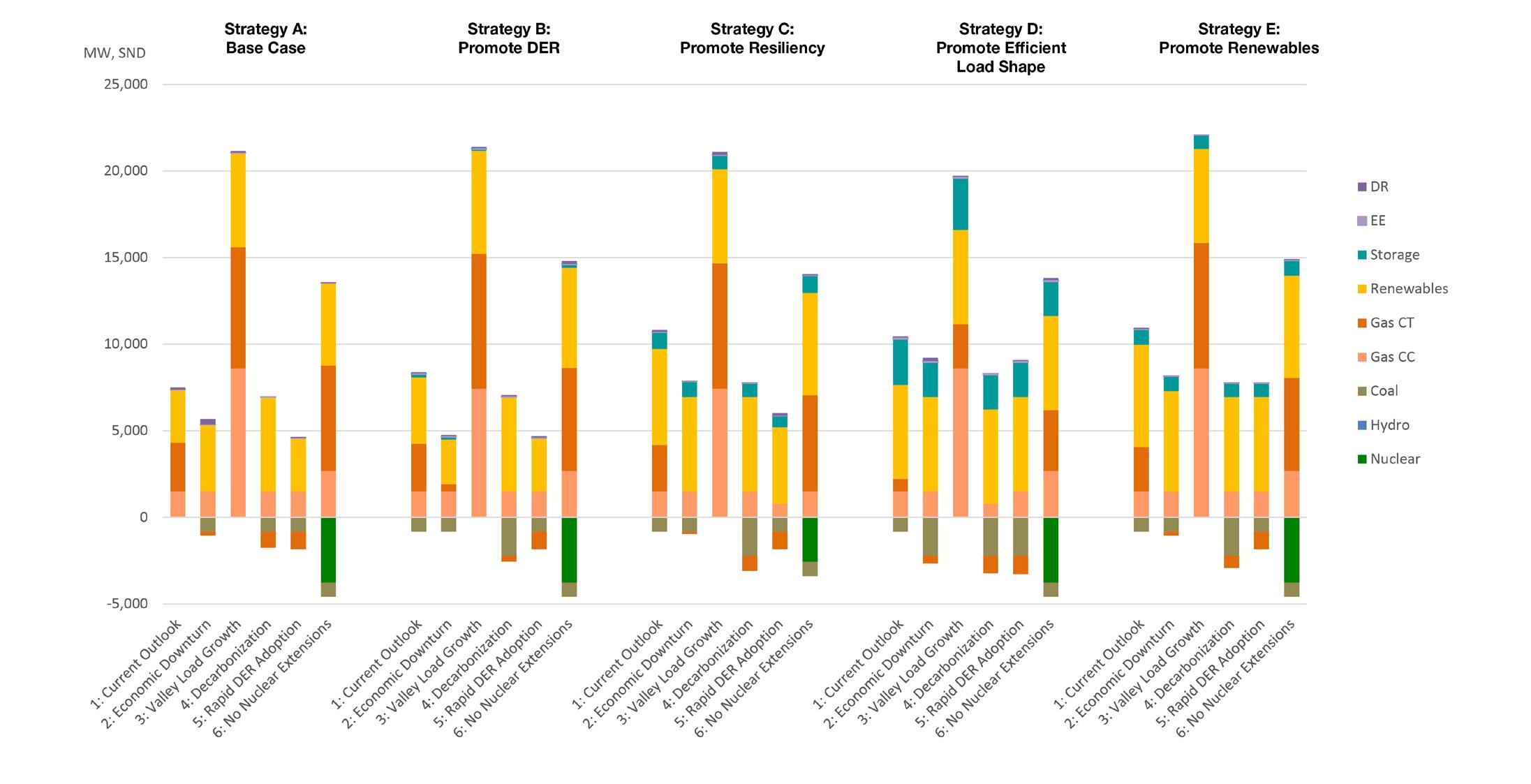
• MWs are incremental additions from 2019 forward. Board-approved coal retirements are excluded from the totals.
• Browns Ferry Nuclear Plant license is not extended in the No Nuclear Extensions Scenario (outside of TVA control).
• Upper bounds of potential natural gas and solar additions are driven by the Valley Load Growth Scenario.
• Solar and wind are shown in nameplate capacity; accelerated solar additions are reflected in the IRP Recommendation.
• Solar, gas, and storage ranges include utility-scale and distributed additions (where promoted in a strategy).
TVA’s recommended planning direction affirms its commitment to a diverse and flexible resource portfolio guided by the leastcost system planning mandate. The ranges shown, stated in megawatts (MW) of capacity, provide a general guideline for resource selections. In developing a Recommendation from the study, TVA elected to establish guideline ranges for key resource types (owned or contracted) that make up the target power supply mix. This general planning direction is expressed over the 20-year study period while also including more specific direction over the first 10-year period. Meeting the Valley’s future needs in accordance with the resource technologies and ranges in this Recommendation will position TVA to continue to deliver low-cost, reliable and clean power to the people of the Tennessee Valley.


Coal: Continue with announced plans to retire Paradise in 2020 and Bull Run in 2023. Evaluate retirements of up to 2,200 MW of additional coal capacity if cost-effective.
Hydro: All portfolios reflect continued investment in the hydro fleet to maintain capacity. Consider additional hydro capacity where feasible.


Energy Efficiency: Achieve savings of up to 1,800 MW by 2028 and up to 2,200 MW by 2038. Work with our local power company partners to expand programs for low-income residents and refine program designs and delivery mechanisms with the goal of lowering total cost.
Demand Response: Add up to 500 MW of demand response by 2038 depending on availability and cost of the resource.
Nuclear: Pursue option for second license renewal of Browns Ferry for an additional 20 years. Continue to evaluate emerging nuclear technologies, including small modular reactors, (SMR) as part of technology innovation efforts.

Wind: Existing wind contracts expire in the early 2030s. Consider the addition of up to 1,800 MW of wind by 2028 and up to 4,200 MW by 2038 if cost-effective.

Storage: Add up to 2,400 MW of storage by 2028 and up to 5,300 MW by 2038. Additions may be a combination of utility and distributed scale. The trajectory and timing of additions will be highly dependent on the evolution of storage technologies.

Gas Combustion Turbine: Evaluate retirements of up to 2,000 MW of existing combustion turbines if cost-effective. Add up to 5,200 MW of combustion turbines by 2028 and up to 8,600 MW by 2038 if a high level of load growth materializes. Future CT needs are driven by demand for electricity, solar penetration, and evolution of other peaking technologies.

Gas Combined Cycle: Add between 800 and 5,700 MW of combined cycle by 2028 and up to 9,800 MW by 2038 if a high level of load growth materializes. Future CC needs are driven by demand for electricity and gas prices, as well as by solar penetration that tends to drive CT instead of CC additions.

Solar: Add between 1,500 and 8,000 MW of solar by 2028 and up to 14,000 MW by 2038 if a high level of load growth materializes. Additions may be a combination of utility and distributed scale. Future solar needs are driven by pricing, customer demand, and demand for electricity.
The IRP Recommendation meets the dual objective of ensuring flexibility to respond to the future while providing guidance on how our resource portfolio should change as the future unfolds.
With the implementation of the IRP Recommendation will come certain challenges. For example, the IRP Recommendation includes significant renewables expansion, which means it will become increasingly important to know the location of renewable resources, both utility and distributed scale, and how weather impacts solar generation. Early experience with battery storage on the system would provide additional insight to how the various storage-use cases might be employed to provide economic benefit and system flexibility, especially with increasing penetration of renewables. TVA will need to partner with local power companies and other stakeholders in the region to better understand the potential for distributed resources in the Valley and their locational value to inform resource decisions. Finally, the IRP Recommendation also includes more conventional resources, primarily gas-fired, and TVA will need to consider the implementation challenges in the areas of siting and permitting, both for the units themselves and associated transmission lines and gas pipelines.
In the process of developing the IRP, stakeholders raised a number of policyrelated issues that are outside the scope of the IRP itself but will need to be considered as TVA moves toward implementation of recommendations from the IRP study. These considerations include continued evolution of programs that provide flexibility for customerowned generation, evolution of federal/ state energy and environmental policies, advancements in customer expectations and requirements for clean energy, and enhancing low-income equity and energy/environmental justice.
The scenarios and strategies evaluated in the IRP provide insights to how TVA’s resource portfolio may need to evolve as the future becomes clearer. The results indicate there are near-term actions that would provide benefit across multiple futures. The actions include:


• Add solar based on economics and to meet customer demand.
• Enhance system flexibility to integrate renewables and distributed resources.
• Evaluate demonstration battery storage to gain operational experience.
• Pursue option for license renewal for TVA’s nuclear fleet.
• Evaluate engineering end-of-life dates for aging fossil units to inform long-term planning.
• Conduct market potential study for energy efficiency and demand response.
• Collaborate with states and local communities to address low-income energy efficiency.
• Collaboratively deploy initiatives to stimulate the local electric vehicle market.
• Support development of Distribution Resource Planning for integration into TVA’s planning process.
As the future unfolds, TVA will monitor key signposts that will guide decisions in the longer term. The signposts relate to key variables that could have a significant influence on the future generation portfolio. These key signposts include:
Developing the 2019 IRP has been an approximately 18-month process that began in February 2018 and will conclude when a Record of Decision is released. The IRP process will have included the following activities:
• Scoping, which took place in winter/spring 2018 and identified issues important to the public and laid the foundation for developing the IRP.
• Development of Model Input and Framework, which occurred in spring/summer 2018 and included identifying and developing scenarios, resource options and business strategies to evaluate how a future portfolio might change under different conditions.
• Analysis and Evaluation, which took place in fall 2018 and included developing and evaluating the performance of the 30 resource portfolios.
• Presentation of Initial Results, which occurred in February 2019 with release of the draft IRP and EIS.
• Public Comment Period, which was held from February 15 to April 8, 2019.
• Additional Analysis, which was completed in response to stakeholder and public comments.
• Completion of the Study , which includes the IRP Recommendation, near-term actions and key signposts, and the final environmental assessment.
• Publication of the Final IRP and EIS on June 28, 2019, on TVA’s website.
• Expected Request for Approval of the IRP Recommendation from the Board in August 2019.
TVA will closely monitor these key drivers related to changing market conditions, more stringent regulations, and technology advancements to inform appropriate actions within the recommended ranges and appropriate timing for initiating the next IRP.
• Record of Decision will be published after Board approval.
With input from the IRP Working Group, TVA designed scenarios that are outside of TVA’s control but represent possible futures in which TVA may find itself operating. TVA created a list of uncertainties that could alter the future operating environment and affect the cost of electricity and/or mix of optimal resources. The scenarios are:
With input from the IRP Working Group, TVA developed five strategies, which are business decisions or directions that TVA could employ in each scenario. As it relates to strategies in the IRP, the word “promote” means an incentive was modeled to make the resource more attractive for adoption or selection. The five strategies are :
1
2
SCENARIOS
CURRENT OUTLOOK which represents TVA’s current forecast for these key uncertainties and reflects modest economic growth offset by increasing efficiencies;
ECONOMIC DOWNTURN which represents a prolonged stagnation in the economy, resulting in declining loads (customers using less power) and delayed expansion of new generation;
VALLEY LOAD GROWTH
3
4
which represents economic growth driven by migration into the Valley and a technology-driven boost to productivity, underscored by increased electrification of industry and transportation;
DECARBONIZATION which is driven by a strong push to curb greenhouse gas emissions due to concern over climate change, resulting in high CO2 emission penalties and incentives for non-emitting technologies;
A
5
6
RAPID DER ADOPTION which is driven by growing consumer awareness and preference for energy choice, coupled with rapid advances in technologies, resulting in high penetration of distributed generation, storage and energy management;
NO NUCLEAR EXTENSIONS which is driven by a regulatory challenge to relicense existing nuclear plants and construct new, large-scale nuclear. This scenario also assumes subsidies to drive small modular reactor (SMR) technology advancements and improved economics.
B
STRATEGIES
BASE CASE which represents TVA’s current assumptions for resource costs and applies a planning reserve margin constraint. This constraint applies in every strategy and represents the minimum amount of capacity required to ensure reliable power;
PROMOTE DISTRIBUTED ENERGY RESOURCES
which incents DER to achieve higher, long-term penetration levels. The DER options include energy efficiency, demand response, combined heat and power, distributed solar and storage;
C
PROMOTE RESILIENCY which incents small, agile capacity to maximize operational flexibility and the ability to respond to short-term disruptions on the power system;
PROMOTE EFFICIENT LOAD SHAPE
D
which incents targeted electrification (by incentivizing customers to increase electricity usage in off-peak hours) and demand response (by incentivizing customers to reduce electricity usage during peak hours). This strategy promotes efficient energy usage for all customers, including those with low income;
E
PROMOTE RENEWABLES which incents renewables at all scales (from utility size to residential) to meet growing or existing consumer demand for renewable energy.
TVA uses an industry standard model to derive an optimal capacity plan, considering the focus of each strategy evaluated in each scenario. Modeling assumptions, the framework of IRP planning, are the constraints and planning guidelines that are put into the model. The reliability constraint is especially critical, as it ensures we have enough capacity at all times to provide reliable electricity to customers. For the 2019 IRP, it also is crucial to understand how the system would operate with more renewables and DER on the system –driving a greater need for operational flexibility. TVA considered a broader range of mature and emerging technologies in this IRP, including some distributed energy technologies.
Throughout the IRP process, TVA engaged external stakeholders to understand diverse opinions and to challenge assumptions. TVA established the IRP Working Group, whose 20 members represent diverse interests in the Valley. The IRP Working Group met approximately monthly to review input assumptions and preliminary results and to enable its members to provide their respective views to TVA. TVA also presented IRP progress updates to the Regional Energy Resource Council (RERC), a federal advisory committee that provides advice to the TVA Board of Directors on a range of energy-related matters, including the IRP.
During a 60-day scoping period from February 15 through April 16, 2018, TVA obtained public comments on the scope of the effort to develop this IRP, which helped shape the draft IRP and EIS. After the release of the draft IRP and EIS on February 15, 2019, TVA provided a public comment period through April 8, 2019. TVA held meetings across the Tennessee Valley and an online webinar, and accepted public comments via mail, email, online and in-person at the meetings. Input was critical in shaping the IRP and EIS, and many of the sensitivity analyses that were performed were informed by stakeholder and public input.
The IRP Working Group included representatives from:
• State and local governments
• Academia and research groups
• Advocacy groups
• Local power companies (LPCs)
• Economic development organizations
• Directly-served/ industrial customers
Incremental capacity by 2038 consists of additions of new energy resources and retirement of existing energy resources for the portfolios associated with each strategy.
Total Energy in 2038 by resource type in the portfolios associated with each strategy.
Each IRP case represents a combination of expectations about the future environment TVA operates in and potential strategies TVA could employ that result in unique resource portfolios. The modeling process resulted in 30 resource portfolios. The model analyzed how to achieve the lowest-cost portfolio with each strategy in each scenario, looking for the optimal solution within that particular combination. With input from the IRP Working Group and RERC, TVA identified 14 metrics that reflect desired goals and priorities in areas related to cost, risk, environmental stewardship, operational flexibility and Valley economics. The metrics were used to evaluate tradeoffs among the 30 resource portfolios.
All strategies have similar impacts on the Valley economy as measured by per capita income and employment
When analyzing results from the draft IRP, TVA identified issues that warranted further evaluation prior to finalizing the study. In addition, TVA received helpful input from the IRP Working Group and the RERC, as well as from the public during the comment period. Many of the questions raised by TVA, stakeholders and the public focused on certain key assumptions that could influence results. To explore the impacts of changes in key assumptions and to inform the Recommendation, TVA evaluated sensitivities related to the following categories: natural gas prices; storage, wind, combined heat and power (CHP) and small modular reactor (SMR) capital costs; greater energy efficiency (EE) and demand response (DR) market depth; integration cost and flexibility benefit; pace and magnitude of solar additions; higher operating costs for coal plants; more stringent carbon constraints; and variation in climate.
Summary of 2019 IRP Sensitivities
Note
• Impacts shown in Summer Net Dependable MW, except for solar and wind that are shown in nameplate MW
The IRP results — including the 30 primary cases and the sensitivity cases — provide a robust set of potential resource additions and retirements. The final Recommendation is derived from this evaluation. The Recommendation takes into account customer priorities around power cost and reliability across different futures, along with environmental stewardship and Valley economics considerations. In developing a recommendation from the study, TVA elected to establish guideline ranges for key resource types (owned or contracted) that make up the target power supply mix. In order to distill the considerable number of cases evaluated through the original scenario and strategy analysis and the sensitivity cases, the Recommendation uses ranges that are centered on results obtained under the Current Outlook scenario. The other scenario and sensitivity results provide a sense of how the target power supply mix might change as the future changes. Recognizing that a variety of future scenarios are possible and each strategy has positive aspects, all IRP results are included in the Recommendation to provide flexibility for how the future evolves. Implementing the least-cost resource plan with all of these priorities in mind will help ensure TVA continues to fulfill its mission to serve the people of the Tennessee Valley.
TVA’s EIS assesses the natural, cultural and socioeconomic impacts associated with the 2019 IRP. The five strategies are the basis for the alternatives discussed in the EIS. The Base Case serves as the No-Action Alternative, and the remaining four strategies are the Action Alternatives. The draft EIS analyzed and identified the relationship of the natural and human environment to each of the five alternative strategies. The final EIS includes an additional alternative, the 2019 Recommendation (Target Power Supply Mix). The portfolios associated with each of the five alternative strategies, as well as the 2019 Recommendation, are quantitatively and qualitatively evaluated to determine the environmental impact. This evaluation addresses systemwide topics, including
• Greenhouse gas emissions
• Fuel consumption
• Air quality
• Water quality and quantity
• Waste generation and disposal
• Land requirements
• Socioeconomic impacts
• Environmental justice.
Public comments on the draft EIS and draft IRP are addressed in the final EIS.
The primary study area described in the EIS includes the combined TVA service area; the Tennessee River watershed; and parts of the Cumberland, Mississippi, Green and Ohio Rivers in TVA’s power service area. For some resources, such as air quality and climate change, the assessment area extends beyond the TVA region. For some socioeconomic resources, the study area consists of the 170 counties where TVA is a major provider of electric power and/or operates generating facilities.
Under all the portfolios and the 2019 Recommendation, there is a need for new capacity, with a significant expansion of solar generation overall. Uncertainty around future environmental standards for carbon dioxide emissions, along with the outlook for loads and gas prices, are key considerations when evaluating potential coal retirements. Emissions of air pollutants, the intensity of greenhouse gas emissions (CO 2 intensity) and generation of coal waste decrease under all strategies. Strategies focused on resiliency, load shape and renewables have the largest amounts of solar and storage expansion and coal retirements, resulting in lower environmental impact overall but higher land use. For most environmental resources, the impacts are greatest for the No Action alternative. The exception is the land area required for new generating facilities, which is greater for the action alternatives, particularly strategies which focus on resiliency, load shape and renewables. Most of this land area would be occupied by solar facilities, which, compared to most other energy resources, have a relatively low level of impact to the land. Additional sensitivity analysis showed the potential for an extended range of resource additions and retirements, which generally resulted in reduced impacts to most environmental resources. The land area occupied by solar facilities, however, could greatly increase.
TVA finds considerable value in undertaking an IRP and EIS, and especially appreciates the input, review and insights of individuals on the IRP Working Group and the Regional Energy Resource Council. They spent considerable time helping TVA develop a robust plan that meets all the criteria outlined in its objectives. TVA values their involvement and the expertise they provided on behalf of their respective stakeholders in making this a better IRP.
As with any long-term plan, TVA’s IRP reflects what we know today and can reasonably expect for the coming years. TVA and our employees across the Valley stand ready every day to carry out our three-part mission around energy, the environment and economic development. In an ever-changing world, TVA will do its best to continue to serve the people of the Tennessee Valley by providing low-cost, reliable and clean power in an environmentally responsible manner while promoting economic development across the Valley.
Appendix A – Generating Resource Cost and Performance Estimates
Appendix B – Programmatic Resource Methodology
Appendix C – Distributed Generation Methodology
Appendix D – Modeling Framework Enhancements
Appendix E – Scenario Design
Appendix F – Strategy Design
Appendix G – Capacity Plan Summary Charts
Appendix H – Stochastic Results for Cost Metrics
Appendix I – Method for Computing Environmental Metrics
Appendix J – Method for Computing Valley Economic Impacts
Acronym Description
4th NCA Fourth National Climate Assessment
AC Alternating Current
ACS American Community Survey
APWR Advanced Pressurized Water Reactor
ARC Appalachian Regional Commission
B.P. before present
BART Best Available Retrofit Technology
BCF billion cubic feet
Btu British Thermal Units
CAA Clean Air Act
CAES compressed air energy storage
CAGR compound annual growth rate
CC Combined Cycle
CCR Coal Combustion Residuals
CCS carbon capture and storage/sequestration
CCW condenser cooling water
CEQ Council on Environmental Quality
CFR Code of Federal Regulations
CHP Combined Heat and Power
CO carbon monoxide
CO2 carbon dioxide
CO2-eq CO2-equivalent emissions
CRM Clinch River Mile
CT Combustion Turbine
CWA Clean Water Act
DC Direct Current
DDT Dichlorodiphenyltrichloroethane
DER Distributed Energy Resources
DGIX Distributed Generation Information Exchange
DO dissolved oxygen
DOE Department of Energy
DP Data Profile
DR demand response
DSM Demand Side management
dV deciview
E.O. Executive Order
EA Environmental Assessment
EBCI Eastern Band of Cherokee Indians
EE energy efficiency
Acronym Description
EIS Environmental Impact Statement
EPRI Electric Power Research Institute
ERM Emory River Mile
ESA Endangered Species Act
FERC Federal Energy Regulatory Commission
FGD flue gas desulphurization
FOM Fixed operating and maintenance costs
FY Fiscal Year
gal/d/mi2 gallons per day per square mile
GDP Gross Domestic Product
GHG greenhouse gas
GP Generation Partners
GPP Green Power Providers
GW gigawatt
GWh gigawatt hours
HAP Hazardous Air Pollutants
HFC hydroflurocarbons
Hg Mercury
HUC Hydrologic Unit Code
HVAC heating, ventilation, and air conditioning
HVDC high voltage direct current
IGCC integrated gasification combined cycle
IMP Internal Monitoring Point
IPP Independent power producers
IRP Integrated Resource Plan
KDFWR Kentucky Department of Fish and Wildlife Resources
KPDES Kentucky Pollutant Discharge Elimination System
kV kilovolt
KWh kilowatt-hours
LCA life cycle assessments
LED light emitting diode
LPC Local Power Companies
MAPE Mean absolute percent error
MATs Mercury and Air Toxics Standards
MBCI Mississippi Band of Choctaw Indians
MBTA Migratory Bird Treaty Act
MBtu Million British Thermal Units
MGD million gallons per day
MISO Midcontinent Independent System Operator
MLGW Memphis Light, Gas and Water
MSAs metropolitan statistical areas
MW Megawatt
Acronym Description
MWh Megawatt-hour
N2O Nitrous oxide
NAAQS National Ambient Air Quality Standards
NEPA National Environmental Policy Act
NFIP National Flood Insurance Program
NHPA National Historic Preservation Act
NO2 nitrogen dioxide
NOI Notice of Intent
NPDES National Pollutant Discharge Elimination System
NPS National Park Service
NRC Nuclear Regulatory Commission
NREL National Renewable Energy Laboratory
NRHP National Register of Historic Places
NWS National Weather Service
ORSANCO Ohio River Valley Water Sanitation Commission
PCB polychlorinated biphenyl
PEP Population Estimates Program
PFC perfluorocarbons
PFOS Perfluorooctane sulfonate
PM particulate matter
PPA Power Purchase Agreement
ppm parts per million
PSA Power Service Area
PURPA Public Utility Regulatory Policies Act
PV photovoltaic
PVRR Present Value of Revenue Requirement
PWR Pressurized Water Reactor
QCN Quality Contractor Network
RBI Reservoir Benthic Index
RCP representative concentration pathway
RCRA Resource Conservation and Recovery Act
REC Renewable Energy Certificate
RFAI Reservoir Fish Assemblage Index
RICE reciprocating internal combustion engines
ROD Record of Decision
ROS Reservoir Operations Study
RSO Renewable Standard Offer
SAE Statistically Adjusted End-use model
SCPC supercritical pulverized coal
SCR selective catalytic reduction
SDTSA state-designated tribal statistical areas
SEPA Southeastern Power Administration
Acronym Description
SLR Second License Renewal
SMR small modular reactors
SND summer net dependable
SO2 sulfur dioxide
SOC Special Opportunities Counties
SPCP supercritical pulverized coal plant
SPP Southwest Power Pool
T&D transmission and distribution
TCP Traditional Cultural Properties
TDEC Tennessee Department of Environment and Conservation
TDS total dissolved solids
TRM Tennessee River Mile
TSCA Toxic Substances Control Act
TSS total suspended solids
TVA Tennessee Valley Authority
TWRA Tennessee Wildlife Resources Agency
USACE U S Army Corps of Engineers
USBEA U S Bureau of Economic Analysis
USBLS U.S. Bureau of Labor Statistics
USCB U.S. Census Bureau
USDA U.S. Department of Agriculture
USDOE U.S. Department of Energy
USET United South and Eastern Tribes, Inc.
USFWS U.S. Fish and Wildlife Service
USGS U.S. Geological Survey
VOC volatile organic compounds
VOM Variable operating and maintenance costs
WAP Weatherization Assistance Program
WKWMA Western Kentucky Wildlife Management Area
TVA has developed the 2019 IRP and associated programmatic EIS to address the demand for power in the TVA service area, the resource options available for meeting that demand, and the potential environmental, economic and operating impacts of these options. The IRP will serve as a roadmap for meeting the energy needs of TVA’s customers over the next 20 years.
TVA was created by Congress in 1933 and charged with a unique mission – to improve the quality of life in the Valley through the integrated management of the region’s resources For more than eight decades, TVA has worked to carry out that mission and to make life better for the nearly 10 million people who live, work
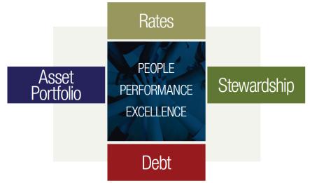
and play in the Valley. TVA is fully self-financed, funding virtually all operations through electricity sales and power system bond financing. TVA sets rates as low as feasible and reinvests net income from power sales into power system improvements and economic development initiatives. TVA makes no profit and receives no tax money. To achieve its overall mission of providing low-cost, reliable power to the people of the Valley, TVA focuses on four strategic imperatives: balancing power rates and debt so that TVA maintains low rates while living within its means; and recognizing the trade-off between optimizing the value of our asset portfolio and being responsible stewards of the Valley’s environment and natural resources (Figure 1-1) Today, TVA continues to serve the people of the Tennessee Valley through its work in three areas: Energy, the Environment and Economic Development.
TVA is the largest producer of public power in the United States. TVA provides wholesale power to 154 local power companies and directly sells power to 58 industrial and federal customers. TVA’s power system serves nearly 10 million people in a seven-state, 80,000-square-mile region (the Valley)
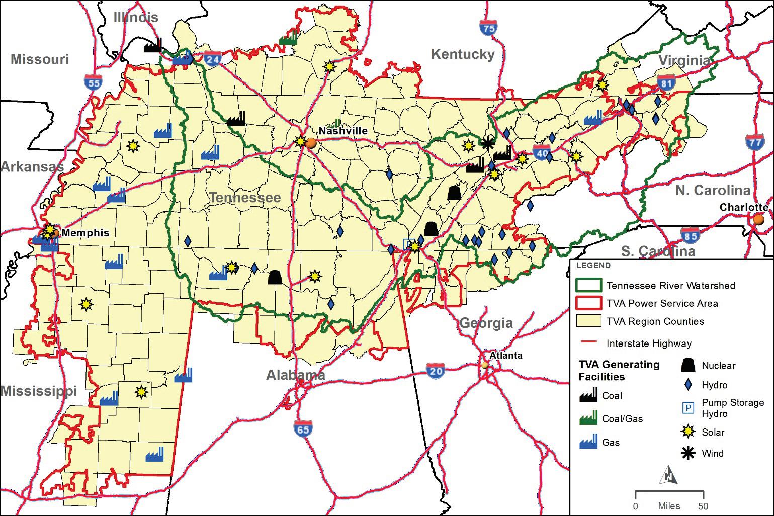
TVA’s generating assets include: six coal plants, three nuclear plants, 29 conventional hydro plants, one pumped storage hydro plant, nine natural gas combustion turbine (CT) gas plants, eight natural gas combined cycle (CC) gas plants, one diesel generator site, and 14 solar sites. TVA has gas-co-firing potential at one coal-fired site as well as biomass co-firing potential at all of its coal-fired sites In total, these
assets constitute a portfolio of 33,500 MWs. TVA also purchases a portion of its power supply from thirdparty operators under long-term power purchase agreements (PPAs).
Safe, clean, reliable and affordable electricity powers the economy of our region and enables greater prosperity and a higher quality of life for everyone. In setting rates, the TVA Board is charged by Section 113 of the Energy Policy Act of 1992 (now the least-cost, system-wide planning provision of the TVA Act) to have due regard for the primary objectives of the TVA Act, including the objective that power be sold at rates as low as are feasible
TVA operates one of the largest transmission systems in the U.S. It serves an area of 80,000 square miles through a network of about 16,200 miles of transmission lines, 500 substations, switchyards and switching stations, and over 1,300 individual customer connection points. The system connects to switchyards at generating facilities and transmits power from them at primarily either 161 kV or 500 kV to local power companies and directly served customers. For the past 18 years, the system has achieved 99.999 percent power reliability. It efficiently delivered nearly 163 billion kilowatt-hours of electricity to customers in FY 2018
Also, the TVA transmission system has 69 interconnections with 13 neighboring utilities at interconnection voltages ranging from 69-kV to 500-kV. These interconnections allow TVA and its neighboring utilities to buy and sell power from each other and to wheel power through their systems to other utilities. To the extent that Federal law requires access to the TVA transmission system, the TVA transmission organization
offers services to others to transmit power at wholesale in a manner that is comparable to TVA's own use of the transmission system, according to FERC Standards of Conduct for Transmission Providers (FERC 2008)
In recent years, TVA has built an average of 75 miles of new transmission lines and several new substations and switching stations per year to serve new customer connection points and/or to increase the capacity and reliability of the transmission system. TVA has also upgraded many existing transmission lines. A major focus of recent transmission system upgrades has been to maintain reliability when coal units are retired. Between 2011 and 2018, TVA spent about $420 million on these upgrades and anticipates spending $10 million on coal-retirement related transmission system upgrades in 2019 and 2020. The upgrades include modifications of existing lines and substations and new installations as necessary to provide adequate transmission capacity, maintain voltage support, and ensure generating plant and transmission system stability. In May 2017, TVA began a $300 million, multiyear effort to upgrade and expand its fiber-optic network to help meet the power system’s growing need for bandwidth as well as accommodate the integration of new distributed energy resources.
Additionally, TVA makes annual investments in science and technology innovation that enable TVA to meet future business and operational challenges Core research activities directly support improving generation and delivery assets, enhancing air and water quality, and integrating clean energy resources
Environmental stewardship is an important part of TVA’s mission of service TVA is committed to protecting the Valley’s natural resources, as well as its historical and cultural heritage. TVA manages and monitors 293,000 acres of reservoir land, 11,000 miles of shoreline and 80 public recreation areas. These areas generate about $12 billion a year in recreation to the regional economy and create or retain about 130,000 jobs each year
To protect water quality and aquatic life, TVA has installed equipment to add oxygen to the water around TVA dams and committed to releasing minimum flow to keep the downstream riverbed from drying out when power generation is shut off.
To protect air quality, TVA has invested nearly $7 billion installing systems to reduce nitrogen oxides and sulfur dioxide emissions from coal-fired plants. TVA has also reduced carbon dioxide emissions by retiring several of its oldest, least efficient coal-fired units and adding cleaner forms of power generation, including:
• the first nuclear unit of the 21st century,
• more clean-burning natural gas units,
• generating and purchasing more renewable energy
Through FY 2018, these actions have helped TVA to achieve:
• a 98 percent reduction in sulfur dioxide (SO2) from peak levels in 1977,
• a 94 percent reduction in nitrogen oxides (NOx) emissions from peak levels in 1995,
• reduced water use, wastewater discharges, and waste production from TVA’s operations, and
• a 47 percent reduction in carbon dioxide (CO2) emissions through calendar year 2017 compared to 2005 levels.
Economic development is a cornerstone of TVA’s mission to make life better for Valley residents. In 2018, TVA worked in partnership with communities and the business sector to spur over $11.3 billion in business investments in the Valley, helping to attract and retain more than 65,400 jobs. This was in addition to assisting more than 200 companies to locate or expand existing operations in the Valley. TVA also assisted communities directly with more than 1,100 outreach activities related to economic growth preparedness and retail business development, including 34 communities in the Valley Sustainable Communities Program, which helps to differentiate those communities by highlighting and increasing local sustainability efforts. TVA is also providing ongoing economic development assistance to communities and companies through financial support, technical services, leadership training, market research and other business offerings.
The purpose of the IRP and EIS process is to evaluate TVA’s current energy resource portfolio and alternative future portfolios of energy resource options to meet the future electrical energy needs of the TVA region at a least system-wide cost while taking into account TVA’s mission of energy, environmental stewardship and economic development. The Recommended Target Power Supply Mix described in the 2015 IRP was formally approved by the TVA Board of Directors in August 2015 and has guided TVA decisions since then.
Several recent industry-wide changes have led TVA to begin development of the new IRP and associated EIS ahead of the five-year cycle identified in the 2015 IRP.
Natural gas supplies are abundant and are projected to remain available at lower cost. The electric system load is expected to be flat, or even declining slightly, over the next 10 years. The price of renewable resources, particularly solar, continues to decline. Consumer demand for renewable and distributed energy resources (including distributed generation, storage, demand response and energy services, and energy efficiency programs) is growing. Given these recent changes, the main focus areas of the 2019 IRP are:
• System flexibility,
• Distributed energy resources, and
• Portfolio diversity.
The focus on flexibility in this IRP is multi- faceted. The Valley benefits from a diverse power system that provides flexibility for how the future evolves As the economics of renewables and distributed energy resources continue to improve, operational flexibility will be increasingly important to successfully integrate these resources into the generation portfolio. Due to their intermittent nature, TVA needs flexible resources that can quickly respond to dynamic loads.
The following objectives guide the development of this IRP:
• Deliver a plan aligned to mandated least-cost planning principles,
• Ensure the portfolio delivers energy in a reliable manner,
• Manage risk by utilizing a diverse portfolio of supply and demand-side resources,
• Deliver cleaner energy and continue to reduce environmental impacts,
• Evaluate increased use of renewables, energy efficiency, and distributed energy resources,
• Continue to innovate by dynamically modeling energy efficiency and distributed energy resources in the study,
• Proactively plan to meet future needs for system flexibility,
• Provide flexibility to adapt to changing market conditions and identify significant signposts,
• Increase credibility and trust through a collaborative and transparent process, and
• Integrate stakeholder perspectives throughout the study
Given these objectives and in consideration of the focus areas listed above, the final, optimal resource plan has been developed with the goals of being lowcost, risk-informed, environmentally responsible, reliable, diverse, and flexible.
TVA developed this new IRP and associated EIS to proactively address several changes within the utility marketplace, both regionally and nationally Upon adoption by the TVA Board, the IRP will replace the 2015 IRP. The purpose of the IRP and EIS processes is to evaluate TVA’s current energy resource portfolio and alternative future portfolios of energy resource options to meet the energy needs of the Valley while taking into account TVA’s mission of energy, environmental stewardship and economic development.
To ensure TVA best meets projected future needs, TVA has continued its tradition of incorporating innovations in each succeeding IRP.
• The 2011 IRP focused on diversifying and modernizing its generation portfolio, part of which included adding cost-effective renewables.
• The 2015 IRP identified distributed energy resources (DER) as a growing trend in the utility industry and designed a mechanism where energy efficiency could be chosen as a resource.
• The 2019 IRP:
o Improves TVA’s understanding of the impact and benefit of system flexibility to meet dynamically changing loads with increasing renewable and distributed resources.
o Explores various DER scenarios, considering the speed and amount of DER penetration.
o Determines the implications of implementing the selected diverse portfolio mix over the next 20 years.
Distributed energy resources (DER) are power generation and storage systems that are connected to the power distribution system and deliver power to the grid or that are “behind the meter” and deliver power directly to an end- user. Examples include solar panels, combined heat and power systems, microturbines, and battery storage systems. DER also includes energy management, such as energy efficiency and demand response.
Building upon previous versions of the IRP, the 2019 IRP includes modeling refinements, updated studies, and additional public outreach. The purpose of these innovations is to provide an IRP that evolves with the industry and helps TVA continue to provide reliable, clean power at the lowest feasible rate
TVA’s planning reserve margin, which provides reserve capacity for unplanned events, has historically been an annual target based on a study focused on the summer peak. In the 2015 IRP, TVA’s planning reserve margin was 15 percent applied across the year. TVA has a dual-peaking system, with similarly high demand in both winter and summer. In winter, there is increased thermal and hydro generating capacity but also greater weather-driven peak variability than in the summer While solar capacity additions are expected, driven by increasing consumer demand and decreasing prices, solar generation does not coincide with winter peak demand times Since the 2015 IRP, TVA conducted an updated reserve margin study to evaluate seasonal differences in demand and supply and the impact of increasing solar capacity on the system. The objective was to identify discrete reserve margin targets for summer and winter to ensure an industry best-practice level of reliability across both peak seasons. The study
also evaluated the cost of reserves and reliability events to the customer. Based on the study, the planning reserve margins being applied in the 2019 IRP are 17 percent for the summer peak season and 25 percent for the winter peak season.
With increasing penetration of variable energy resources, such as wind farms, utility-scale solar farms and rooftop solar, utilities need to ensure their bulk system is flexible enough to respond to dynamically changing loads, even to load changes within each hour. If variable energy resources are added, the balance of the system must respond to their variability, driving an integration cost. Conversely, if very flexible assets (i.e., those that can rapidly change their output) are added, there is a benefit resulting from the balance of the system running more efficiently. To capture these impacts in long-term planning, TVA recently conducted a study to quantify an integration cost for solar and wind resources and a flexibility benefit for small, agile gas and storage resources. The result is a sub-hourly integration cost or flexibility benefit that was applied to energy or build costs in 2019 IRP modeling performed at an hourly level
In the 2015 IRP, DER was included in the load forecast as a load modifier that reduced demand for electricity from TVA, and energy efficiency and demand response were modeled as selectable resources. In the 2019 IRP, TVA made further refinements in modeling behindthe-meter generation in the load forecast, including variations across the scenarios We also modeled distributed generation resources, including combined heat and power, and distributed solar and storage. There are targeted levels of adoption of these distributed resources based on incentive levels in each strategy.
Building upon the outreach and engagement work done for the 2015 IRP, TVA developed an outreach strategy to foster broader engagement from different demographic groups; a social media campaign designed to engage various audiences; and ongoing
communications about the IRP, rather than communications only at key milestones.
Social media communications included multiple posts targeted to the different demographic groups on platforms such as Twitter, LinkedIn, Facebook and Instagram. Additionally, TVA published videos to build the public’s knowledge and understanding of the electrical system as well as the IRP process. Additional details on social media outreach are located in Section 3.3.1 of Volume I.

In conjunction with the issuance of the draft IRP and EIS documents for public review, TVA developed an interactive report to enable members of the public to learn about and provide comments on the draft IRP and EIS documents. Materials from public meetings that TVA hosted across the Valley are also on TVA’s IRP webpage. The interactive report has been updated to capture final results.
Volume I contains the 2019 IRP along with descriptions on the methodology and development of the recommendation This works in conjunction with Volume II, which contains the EIS The EIS is an assessment conducted under the National Environmental Policy Act (NEPA) that describes the
environmental effects of a proposed action and its alternatives that may have a significant effect on the quality of the human environment
TVA developed the draft IRP and EIS and made them available to the public and government agencies for review and comment from February 15th, 2019, until April 8th, 2019. During the public comment period, TVA
conducted public meetings across the Valley to discuss the IRP process, share draft results, and receive comments on the draft IRP and EIS Over 1,200 people commented on the draft IRP and EIS. TVA considered all comments received, made revisions as appropriate, and is now publishing the final IRP and EIS The final EIS includes TVA’s responses to public comments on the Draft IRP and EIS.
TVA’s 2019 IRP process consisted of seven distinct steps:
1. Scoping
2. Develop Study Inputs and Framework
3. Analyze and Evaluate
4. Present Initial Results and Gather Feedback
5. Incorporate Feedback and Perform Additional Modeling
6. Identify Preferred Target Supply Mix
7. Approval of IRP Recommendations by TVA Board of Directors
Public participation was integral to the process and is explained in more detail in Chapter 3. Steps 2 through 6 are explained in more detail in Chapter 6
The IRP team collected information from TVA’s resource planning, forecasting, and electricity generation experts to begin developing IRP model inputs. A 60-day public scoping period for TVA’s 2019 IRP occurred from February 15 to April 16, 2018. The objective in this initial step was to identify resource options, strategies and future conditions that merited evaluation in the IRP process Public scoping comments covered a wide range of issues, including the nature of the integrated resource planning process, preferences for various types of power generation, input on planning scenarios and strategies, and the environmental impacts of TVA’s power generation The comments received helped to identify issues important to the public and to lay the foundation for the EIS that supports the 2019 IRP. Additional information on the scoping process and results can be found in Volume I, Section 3.1.
When developing a long-term plan for a power system, utilities typically use a least-cost decision making framework that focuses on a single view of the future. TVA also uses a least-cost decision making framework but considers multiple views of the future to determine how potential resource portfolios could perform across multiple futures given different market and external conditions
TVA’s goal is to identify an energy resource plan that performs well under a variety of future conditions (e.g., a strong economy or a weak economy), thereby reducing the risk that a selected strategy or plan would perform well under one set of future conditions, but poorly under a different set of conditions. This increases the likelihood that TVA’s plan will provide least-cost solutions to future demands for electricity from its power system regardless of how the future plays out.
This decision-making framework requires use of a scenario planning approach Scenario planning provides an understanding of how the results of nearterm and future decisions would change under different conditions over a 20-year planning horizon.
After review of the scoping comments, suggestions from members of the IRP Working Group (see Volume I, Section 3.2), and further analysis, TVA selected the five unique scenarios summarized in Table 2-1. In addition to these five scenarios, TVA also analyzed an additional Current Outlook scenario based on TVA’s current assumptions about future conditions.
Scenarios are alternate plausible futures outsid e of TVA's control with different economic and regulatory conditions, as well as social trends and pace of adoption of newer technologies. Strategies are alternate business approaches within TVA's control that differ in the type and amount of resources tha t are promoted in the future. A portfolio is the result of a strategy evaluated inside a scenario. Each strategy and scenario combination will result in a 20 - year resource portfolio to meet the energy needs of the Valley.
Scenario Description
1- The Current Outlook
2- Economic Downturn
3- Valley Load Growth
4- Decarbonization
5- Rapid DER Adoption
6- No Nuclear Extensions
TVA’s current forecast for key uncertainties that reflects modest economic growth offset by impact of increasing efficiencies resulting in a flat load outlook
Represents a prolonged stagnation in the economy, resulting in declining loads and delayed expansion of new generation
Represents economic growth driven by migration into the Valley, a technology-driven boost to productivity, and increased electrification of transportation
Represents a strong push to curb GHG emissions due to concern over climate change, resulting in high CO2 emission penalties and incentives for non-emitting technologies
Represents growing consumer awareness and preference for energy choice, coupled with rapid advances in technologies driving high penetration of distributed generation, storage, and energy management
Represents a regulatory challenge to relicensing of existing and construction of new, large scale nuclear and a preference for more secure, modular, and flexible technologies, including subsidies to drive a breakthrough in Small Modular Reactor design and cost
After review of the scoping comments, suggestions from members of the IRP Working Group, and further analysis, TVA selected five distinct strategies, including a base case representing least-cost planning with no specific resources promoted and reflecting decisions made to date by the TVA Board of Directors. The resource strategies TVA evaluated are shown in Table 2-2. These strategies differ in their emphasis on
Strategies
A- Base Case
B- Promote DER
C- Promote Resiliency
D- Promote Efficient Load Shape
E- Promote Renewables
distributed generation, energy efficiency and demand response efforts, renewable energy resources, nuclear generating capacity additions, and coal-fired generation. The alternative strategies were analyzed in the context of six different scenarios (Table 2-1) that described plausible future economic and regulatory conditions, as well as social trends and adoption of newer technologies
• Represents TVA’s current assumptions for resource costs and applies a planning reserve margin constraint, which also applies in every strategy
• Promotes DER to high long-term penetration levels by incenting distributed solar and storage, combined heat and power, energy efficiency and demand response
• Promotes small, agile capacity to increase operational flexibility of TVA’s power system, while also improving the ability to respond locally to short-term disruptions
• Promotes targeted electrification, demand response, and energy management to optimize load shape, including programs targeting low-income energy efficiency
• Promotes renewables at all scales to meet growing prospective or existing customer demands for renewable energy
After the resource planning scenarios and strategies were developed, the performance of each planning strategy was analyzed in detail across all of the scenarios. This phase of the IRP used industry standard capacity expansion planning and production cost-modeling software to estimate the total cost of
each combination of strategy and scenario Metrics, financial risks and environmental impacts were developed from the cost-modeling results.
Unique resource plans, or “portfolios,” were developed, one for each combination of scenario and strategy. Each of the 30 portfolios represented a long-term,
least-cost plan of different resource mixes that could be used to meet the region’s power needs.
Every portfolio was evaluated using metrics within a consistent, standard scorecard. The metrics were chosen based on importance to TVA’s mission, and captured financial, environmental, operational and economic impacts. Portfolios were analyzed for their robustness under stress across multiple scenarios and metrics TVA identified portfolios that performed best overall, and those strategies that performed well in most models of the future.
The draft 2019 IRP and EIS were released for public review and comment from February 15th, 2019, until April 8th, 2019 It presented an initial range of viable planning strategies for further consideration, and included scorecards and assessments using key metrics, along with an assessment of environmental impacts based on the draft results. As in the scoping period, TVA encouraged public comments on the draft IRP and associated EIS. Over 300 comment submittals were received, along with a petition from the Sierra Club signed by close to 1,000 individuals. The comments expressed public concerns, questions, and recommendations for the future operation of the TVA power system.
Following the public comment period, all comments were reviewed Similar comments were combined into a group, as appropriate. TVA provided responses to all substantive comments either by revising the IRP or associated EIS, or by providing specific answers in the final EIS. Results of any additional technical analysis conducted to respond to comments are included in the final IRP. Comments received, along with TVA’s responses, can be found in Appendix F of the Final EIS.
After consideration of IRP Working Group and RERC input, review of the public comments received and additional analysis, TVA identified a target power supply mix based on planning strategies evaluated in the IRP. This target, expressed in ranges, reflects the mix of supply and demand side resources that best position the Valley for success in a variety of alternative futures while preserving the flexibility necessary to respond to uncertainty. Final results and implementation considerations are found in Chapter 9 of the IRP.
Considering the IRP key findings and Recommendation for the target power supply mix over the next 20 years, TVA also identified near-term actions that would provide benefit across multiple futures. Additionally, we have highlighted key signposts, or drivers, that will guide decisions in the longer term.
A Notice of Availability of the final 2019 IRP and EIS has been published in the Federal Register No sooner than 30 days after publication of the Notice of Availability in the Federal Register, the TVA Board of Directors will be asked to approve the recommendations included in the study, including the target power supply mix. The Board will decide whether to approve the recommendations presented in the study, to modify them or to approve an alternative. The Board’s decision will be described and explained in a Record of Decision.
Understanding the varying needs and priorities of TVA’s nearly 10 million stakeholders and striking a balance can be challenging, but is a key to TVA’s IRP process Gaining that perspective is why TVA used a transparent and participatory approach in developing this longrange plan. Obtaining diverse input and support for the IRP was one of the goals TVA wanted to ensure those who wanted to participate could do so.
TVA’s public involvement goals were to:
• Engage numerous stakeholders with differing viewpoints throughout the process.
• Incorporate public opinions into the development of the IRP by offering stakeholders and the public opportunities to review and comment on various inputs, analyses and options being considered.
• Encourage open and honest communication in order to provide a sound understanding of the process
• Create public awareness and opportunities to receive feedback.
• Incorporate input from an IRP Working Group and the RERC, made up of people representing the broad perspectives of those who live and work in the Valley.
Public involvement was a particular focus throughout the IRP process described in Section 2, including steps 1 and 2, Scoping and Develop Study Inputs and Framework, and as part of step 4, Present Initial Results and Gather Feedback.
To begin the 2019 process, TVA published a Notice of Intent (NOI) in the Federal Register announcing plans to prepare an EIS to address the potential environmental effects associated with the implementation of the updated IRP. The NOI initiated a 60-day public scoping period starting on February 15, 2018, and ending on April 16, 2018. The NOI included five scoping questions for consideration.
• How do you think energy usage will change in the next 20 years in the Tennessee Valley Region?
• Should the diversity of the current power generation mix (e.g., coal, nuclear, power, natural gas, hydro, renewable resources) change? If so, how?
• How should Distributed Energy Resources (DER) be considered in TVA planning?
• How should energy efficiency and demand response be considered in planning for future energy needs? And how can TVA directly affect electricity usage by consumers?
• How will the resource decisions discussed above affect the reliability, dispatchability (ability to turn on or off energy resources) and cost of electricity?
In addition to the NOI in the Federal Register, TVA sent notification of the NOI to local and state government entities and federal agencies; issued a news release to media; and posted the news release on the TVA website. TVA sent 2,500 scoping notices via email and/or mail to agencies, organizations and the public, including those on the 2015 IRP mailing list and people who registered to receive additional information on the TVA IRP website.
TVA published notices regarding the NOI in local newspapers, including the following cities and associated newspapers.
• Chattanooga, Tenn. – Chattanooga Times Free Press
• Huntsville, Ala – The Huntsville Times
• Memphis, Tenn. – The Commercial Appeal
• Nashville, Tenn. – The Tennessean
• Knoxville, Tenn. – Knoxville News Sentinel
• Paducah, Ky – Paducah Sun
• Bowling Green, Ky – Bowling Green Daily News
TVA maintains a distribution list of more than 2,000 individual stakeholders that is regularly updated with contact information This list includes those who made
public comments, registered on the TVA IRP website, or attended webinars and meetings.
TVA held two public meetings and a public webinar as part of the scoping period:
• February 21, 2018: Webinar
• February 27, 2018: Educational open house at The Westin Chattanooga, 801 Pine St., Chattanooga, Tenn.
• March 5, 2018: Educational open house at Memphis Light, Gas and Water Auditorium, 220 S. Main St., Memphis, Tenn.
The purpose of the scoping period and meetings was to present TVA’s project objectives and initial alternatives for input from the public and interested stakeholders. At each meeting, TVA staff described the process of developing the IRP and associated EIS and responded to questions from meeting attendees both in person and online. Scoping meeting and webinar
materials are included in the Scoping Report on TVA’s website: www.tva.com/irp
Participants included the public; congressional, state and local officials; representatives from local power companies; non-governmental organizations and other special interest groups; and TVA employees.
Ninety-one people attended the meetings in person or via webinar
TVA published the 2019 IRP Scoping Report on August 1, 2018. The Scoping Report includes copies of scoping materials and comments received during the 60-day comment period. TVA received a total of 87 comment submissions Comments were received from six of the seven states within the TVA power service area, with approximately 50 percent from the state of Tennessee. Comments were also received from the District of Columbia and eight states outside of the TVA power service area
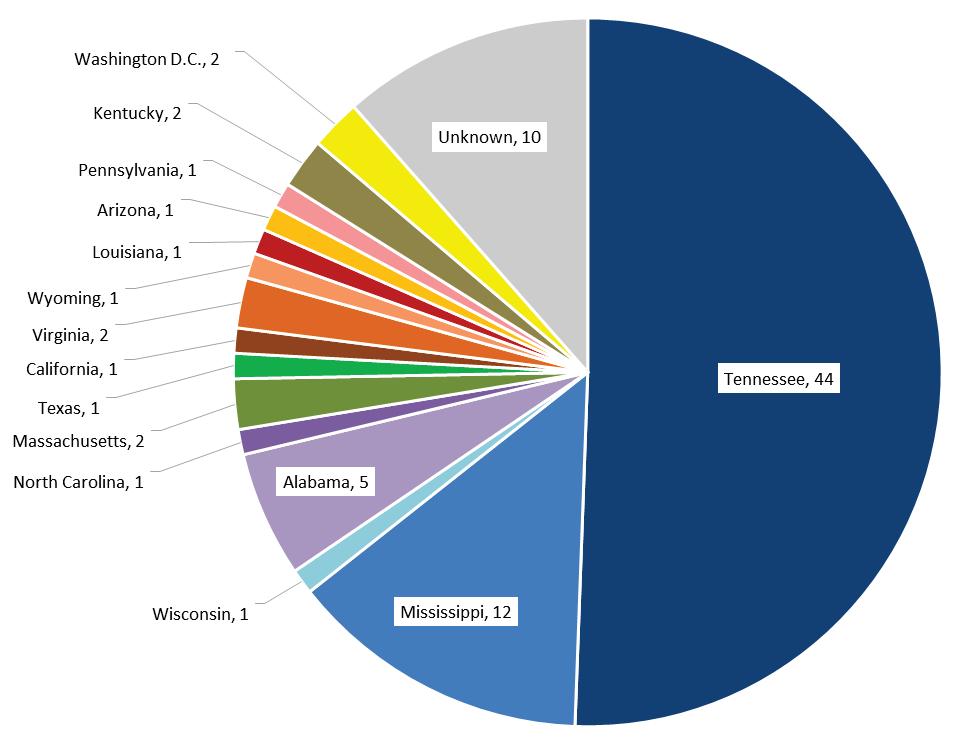
Of the 87 comment submissions, 30 were received from individuals, 28 were from businesses, 23 comments were from civic or non-governmental organizations, four were from government agencies, and two comments were from educational institutions. TVA used scoping comments to develop a list of Frequently Asked Questions, which can also be found on TVA’s website: www.tva.com/irp
Comment Theme
Integrated Resource Planning
Energy Resource Options
Planning Scenarios
Examples of Comments
• Planning process in general.
The information collected during the public scoping period helped shape the initial framework of TVA’s 2019 IRP and was used to help determine which resource options should be considered. Scoping comments, including those from the scoping meetings, addressed a wide range of IRP-related topics categorized as follows.
• TVA’s reason for developing a new IRP.
• Recommendation to include grid reliability and cybersecurity as part of the IRP model.
• Recommendations related to renewables modeling and battery storage.
• Questions about TVA’s flat or declining growth projections in comparison to population and industrial growth in the Valley.
• Emphasis on the use of least-cost analysis and that TVA be sensitive to the adopted plan’s effects on ratepayers.
• Benefits and/or drawbacks of energy options, including nuclear, coal-fired, and natural gasfired generation, as well as solar, biomass, and wind renewable generation and energy storage.
• Recommendations for increased energy efficiency efforts
• Recommendations for increasing demand-reduction options, including demand response and combined heat and power.
• Recommendations for TVA to continue purchasing power from the Red Hills Power Plant. Recommendations to either incentivize or limit the adoption of DER.
• Recommendations that TVA evaluate renewable energy, carbon policy and electrification as potential scenarios
• Recommendation that TVA consider repeal of the Clean Power Plan and Coal Combustion Residual (CCR) disposal rules
Planning Strategies/Alternatives
Portfolio Evaluation Metrics
Environmental Impact Statement
• Recommendations that TVA consider strategies that evaluate energy efficiency, renewable energy and DER.
• Suggestions for portfolio evaluation metrics related to wildlife and recreation benefits, flexibility and resiliency, and low-income and minority communities.
• Questions and comments about the scope of the EIS
• Comments about how TVA should analyze the cumulative impacts of the IRP on various resources.
• Recommendations that TVA provide a detailed evaluation of impacts to low-income and minority communities.
• Various comments about biological resources, air quality, climate and greenhouse gases, and water resources.
Many comments were received about the scope of the EIS and how TVA should analyze the cumulative impacts of the IRP on various resources. In particular, several comments were received recommending TVA provide a detailed evaluation of impacts to low-income and minority communities. Specific comments were also received about biological resources, air quality, climate and greenhouse gases, and water resources.
All of the scoping comments are detailed in the 2019 IRP Scoping Report on TVA’s website.
The formation of an IRP Working Group was a cornerstone of the public input process for the 2019 IRP, just as it was for the 2015 study. Working Group members reviewed input assumptions, preliminary results and provided feedback throughout the process. They provided their individual views to TVA, as well as representing and keeping their constituencies informed regarding the IRP process.
The 2019 Working Group consisted of 20 external stakeholders representing 20 organizations. Eight of the members represented the interests of entities purchasing power from TVA:
• Local power companies (LPCs) (3)
• Industrial customers (3)
• Organizations representing LPCs and industrial customers (2)
The 12 other members represented the following interest groups:
• Energy and environmental non‐governmental organizations (3)
• Research and academia with expertise in DERs (3)
• State government (2)
• Economic development organizations (2)
• Community and sustainability interests (2)
Beginning in February 2018, TVA met with the IRP Working Group approximately every month. Ten meetings were held at various locations throughout the region prior to the release of the draft IRP and
associated EIS, with an additional four meetings held before the release of the final IRP and associated EIS
The meetings were designed to encourage discussion on all facets of the process and to facilitate information sharing, collaboration and expectation setting for the IRP. IRP Working Group members reviewed and commented on proposed scenarios, planning assumptions, analytical techniques, energy resource options and strategies, along with draft results. Specific topics included load and commodity forecasts, resource planning framework, resource options, and energy efficiency and DER approach in the IRP models
Given the diverse makeup of the IRP Working Group, there was a wide range of views on specific issues, such as the value of DER and EE programs, environmental concerns and the costs associated with various generation technologies. Open discussions supported by the best available data helped improve the IRP Working Group’s understanding of the specific issues.
To increase public access to the IRP process, all nonconfidential IRP Working Group meeting material was posted on TVA’s website, along with webinar recordings and related presentation materials
Kendra Abkowitz
State of Tennessee Nashville, Tenn.
Dr. Al Armendariz
Sierra Club Beyond Coal Campaign Tampa, FL
Rick Bender
Commonwealth of Kentucky Frankfort, Ky.
Dr. Don Colliver
University of Kentucky Lexington, Ky.
Odell Frye
Associated Valley Industries (AVI) Chattanooga, Tenn.
Erin Gill
City of Knoxville Knoxville, Tenn.
Paul Griffin
Partnership for Affordable Clean Energy Virginia
Keith Hayward
Northeast Mississippi EPA Oxford, MS
Richard Holland
Directly Served Customer Representative Counce, Tenn.
Dana Jeanes
Memphis Light Gas and Water Memphis, Tenn.
Wes Kelley
Huntsville Utilities Huntsville, Ala.
Teja Kurunganti
Oak Ridge National Lab Oak Ridge, Tenn.
Pete Mattheis
Tennessee Valley Industrial Committee Washington, DC
Jon Maynard
Oxford-Lafayette County Economic Development Foundation and Chamber of Commerce Oxford, MS
Susan Hadley Maynor
Greater Memphis Chamber Memphis, Tenn.
Doug Peters
Tennessee Valley Public Power Association (TVPPA) Chattanooga, Tenn.
Patrice Robinson
Memphis City Council Memphis Tenn.
Dr. Charles Sims
Howard H. Baker Jr. Center for Public Policy, University of Tennessee Knoxville, Tenn.
Brian Solsbee
Tennessee Municipal Electric Power Association Nashville, Tenn.
Daniel Tait Energy Alabama Huntsville, Ala.
In addition to the public scoping and IRP Working Group meetings, TVA hosted four webinars during the IRP process to keep the public informed about the progress of the 2019 IRP and EIS.
• Public Update #1, May 15, 2018
• Public Update #2, September 10, 2018
• Public Update #3, February 26, 2019
• Public Update #4, June 5, 2019
At each webinar, TVA staff made a brief presentation, followed by a moderated Q&A session. Topics discussed at the webinars included an introduction to the integrated resource planning process, development of scenarios and strategies, resource options, evaluation metrics, and sensitivity analyses Webinar materials were posted as they became available on the IRP website.
TVA also briefed the public on the IRP process through presentations in public meetings and to local organizations, clubs and associations.
A key priority for TVA’s public outreach is to improve awareness of the IRP process and promote opportunities for public input. During development of the IRP and EIS, TVA used social media communications to inform and educate the public about the IRP and its processes, and to promote opportunities for public input. Social media communications for the 2019 IRP began in June 2018
and used TVA’s four social media platforms: Facebook, Twitter, LinkedIn and Instagram.
Social media communications objectives for the IRP and EIS included:
• Keep various audiences informed throughout the IRP process;
• Foster more informed public input by educating audiences about what an IRP is and why it is important;
• Provide clear, consistent and accurate information about the IRP; and,
• Encourage a diversity of voices to engage in the IRP process.
Examples of content posted to social media include announcements for public webinars and other IRPrelated events; infographics providing basic information on the IRP; educational graphics on resource generation; IRP scenario and strategy descriptions; and announcement of the draft IRP and draft EIS and associated public meetings. TVA also used social media to promote four videos during the IRP about power delivery and the importance of the IRP, the IRP modeling process, opportunities for public input after the release of the draft IRP and draft EIS, and the final portfolio recommendation. Between June 2018 and May 2019, approximately 75 posts were published about the 2019 IRP across all of TVA’s social media platforms. TVA posted updates throughout the public comment period about upcoming meeting dates and reminders to submit comments via the IRP website or interactive report. TVA continued its use of social media during release of the final IRP and EIS, and included information about TVA’s portfolio recommendation.
TVA defined several communication objectives for the 2019 IRP to help build public awareness and engagement in the process Objectives include to:
• Educate various audiences about the IRP and its importance;
• Keep them informed throughout the IRP process;
• Use simple language to explain technical concepts; and
• Gather input and gain buy-in from customers and stakeholders.
Communications methods included the initial public scoping period with public meetings; public webinars to keep the public updated on the IRP development process and provide an opportunity to ask questions; ongoing social media outreach; and public meetings, tabling events and an interactive report corresponding with the IRP public comment period to help build understanding and gain feedback and comments from the public.
TVA also worked to reach a broader, more diverse cross section of the public to ensure there was awareness about the 2019 IRP and to provide opportunities for comments to be made. TVA sought input from existing partners who serve diverse communities regarding the methods that would be most successful in reaching a broader diversity of people Generally, the input received suggested that working through groups and entities that have existing relationships with various diverse communities would be the most successful way to achieve this. Given this input, TVA sought to join existing events where people of greater diversity already were engaged TVA appreciates key partners such as Greenspaces, Habitat for Humanity, TVA Supplier Diversity Alliance, and the TVA Energy Efficiency Information Exchange partners and local power company partners for helping to provide these opportunities.
Further input suggested that make key materials available in Spanish and ensure that the overall language used was clear and not overly technical, where possible. TVA published materials in Spanish and strived to meet the recommendations for using clear, simple wording in IRP materials
TVA provided the draft IRP and EIS for public comment from February 15, 2019, through April 8, 2019. During this time, TVA also held public meetings around the region to provide an opportunity for residents and stakeholders to learn more about the draft IRP and EIS, ask questions and provide general feedback. These information and feedback opportunities are also consistent with our obligations under the National Environmental Protection Act (NEPA). Written comments were also accepted online, mail and email.
Seven public meetings and a public webinar were held around the TVA region during the public comment period.
Date
Location
February 19, 2019 RERC meeting in Murfreesboro, Tenn.
February 26, 2019 Webinar
February 27, 2019 Knoxville, Tenn.
March 18, 2019 Memphis, Tenn.
March 19, 2019 Huntsville, Ala.
March 20, 2019 Chattanooga, Tenn.
March 21, 2019 Nashville, Tenn.
March 26, 2019 Bowling Green, Ky.
At each of these meetings, TVA presented an overview of the draft IRP, followed by a moderated Q&A session supported by a panel of TVA subject-matter-experts. Attendees were able to address comments or questions to the panel. Attendees also had the option to submit written or online comments at the meetings. Written and online comments were also accepted during the full public comment period. Approximately 300 people attended the public meetings in person and 100 people listened to the webinar online.
In addition to these meetings and webinar, TVA also hosted a booth at the Tennessee Environmental Conference in Kingsport, Tennessee, on March 19, 2019.
Verbal and specific written comments enabled TVA staff to identify public concerns and recommendations
concerning the future operation of the TVA power system.
The meetings and opportunities for public input were promoted on all the TVA social media platforms. A fact sheet (in English and Spanish) was distributed to attendees at the meetings and available on the website at www.tva.com/irp. An interactive report of the IRP is accessible online at tvairp.com
Over 1,200 people commented on the draft IRP and draft EIS. Approximately 300 unique comment statements were derived from comment letters received by TVA. The comment statements can be grouped into the following topics:
• Editorial Comments
• Energy Resource Options
• Environmental Impacts
• General Comments
• Integrated Resource Planning
• Out of Scope
As described in Section 2.5 of the IRP, all comments were reviewed and combined with other similar comments, as appropriate. TVA has provided responses to all substantive comments either by revising the IRP or associated EIS, or by providing specific answers in the final EIS. Results of any additional technical analysis conducted to respond to comments has been included in the final IRP. Comments received, along with TVA’s response, can be found in Appendix F of the Final EIS.
Reviewing comments received during the comment period yielded the following general observations:
• TVA should select a plan that is flexible and quickly adapts to changing conditions.
• Concerns that the IRP does not do enough to promote energy efficiency or support TVA’s energy efficiency programs.
• Support for:
o distributed generation
o demand reduction
o energy storage
• Concern over small amount of energy efficiency in portfolios
• Support for and concern about coal plant retirements
• Increased and earlier adoption of renewable energy
• Concerns that TVA has not been aggressive enough in reducing greenhouse gas emissions in light of recent reports from the
Intergovernmental Panel on Climate Change and National Climate Assessment.
• Support for and opposition to nuclear energy
• Concern about the accuracy of land use metric, particularly for solar generation
• Assumptions of costs for various resources
• Need for more transparency in IRP process and benchmarking
• Operations and role of the IRP Working Group.
A primary purpose of this IRP is to determine the optimal mix of resources to supply the power the Tennessee Valley region will need over the 2019 to 2038 study period. TVA estimates the capacity gap by comparing anticipated demand and current supply, and then determines the type and amount of additional generating resources or energy management services needed to fill the gap. TVA would also consider whether retirements of certain resources may be economical, such as in low load cases.
This chapter describes the four steps in the process used to make this determination: estimate demand, determine reserve capacity needs, estimate supply and estimate the capacity gap.
The first step in forecasting future power needs is to estimate long-term growth in electricity sales and seasonal peak demand. Seasonal peak demand, or peak load, is the highest one-hour power requirement placed on the system in a given season, winter or summer. In order to reliably serve customers, TVA must have sufficient resources to meet the peak hour demand.
The electricity sales and peak demand forecasts for this IRP were developed from individual, detailed forecasts of residential, commercial and industrial sales. TVA generated a range of forecasts (high, expected, and low) to ensure that its plans do not depend on the accuracy of a single forecast.
To forecast future electricity demand, TVA uses statistical and mathematical models that link electricity sales to several key drivers. These include the growth in overall economic activity, changes in the underlying demographics, energy substitution and changes in consumer usage through technology
The main forecasting tool TVA utilizes is a Statistically Adjusted End-use model (SAE). This model is designed
to take the changing customer base and usage data into account to produce flexible and dynamic forecasts
As an example, for residential consumers, energy usage is forecasted for space heating, air conditioning, water heating and several other uses after accounting for changes in efficiency over time, appliance saturation and replacement rates, growth in average home size and other factors. Changes in these factors accurately describe the decline in average use per residential customer observed over the last half decade.
Finally, working with its customer service representatives, TVA supplements historical data used in modeling with industry analyses and feedback from large, directly served customers regarding demand. This input helps TVA better predict the magnitude and timing of changes in load attributable to both plant closures and expansions.
On a biannual basis, TVA produces a forecast of regional economic activity for budgeting and longrange planning purposes. These forecasts are developed first on a national basis, which is then filtered into county-level economic forecasts in order to accurately model the prevailing economic conditions in the region.
Historically, the Valley economy has been more dependent on manufacturing than the economies of other regions. Industries such as pulp and paper, aluminum, steel and chemicals were drawn to the Valley because of the availability of natural resources, access to a skilled workforce and the supply of reliable and affordable electricity. However, manufacturing’s share of non-farm employment has steadily declined in the Valley, as it has across the nation
TVA’s region is similar to others in that manufacturing’s share of economic output in the Valley has eased slightly, sliding from 16.6 percent in 2005 to 15.3 percent as of 2017. This contrasts with the U.S. overall, where the manufacturing share of output has declined slightly faster, falling from 13.0 percent to 11.2 percent
during that same timeframe. While many labor-intensive manufacturing industries have moved overseas, a continued shift toward energy-efficient manufacturing processes in the Valley is helping to preserve manufacturing’s contribution to total economic output. This is important to TVA’s load forecasting in that it may indicate a weakening in the historical relationships between economic growth and load growth.
Because of this continued dependence on manufacturing, the region’s economy tends to be more sensitive to economic conditions impacting the demand for manufactured goods. Growth in 2018 and 2019 is expected to benefit from positive cyclical economic conditions. After 2019, however, longer-term demographic pressures are expected to hold average growth in Gross Regional Product near 1.9 percent over the next decade as retiring baby boomers restrict the available labor supply. Population growth in the Tennessee Valley declined from an annual average of about 1.0 percent per year in 1980 to 0.7 percent in 2016. Looking forward, it is expected to steadily decline to around 0.6 percent per year by 2024, further easing to 0.5 percent per year by the tail end of the IRP horizon (2033 – 2038). This will tend to slow the pace of demand increase for all goods and services, including power
Over the past 25 years, the electric utility industry has undergone a fundamental change in most parts of the country. In many states, an environment of regulated monopoly has been replaced with varying degrees of competition. Although TVA has contracts with the 154 LPCs, it is not immune to competitive pressures. The contracts allow LPCs to give TVA notice of contract cancellation after which they may buy power from other sources. Many large industrial customers also have the option of shifting production to plants outside TVA’s service area if TVA’s rates become non-competitive. Additionally, large industrial operations could generate their own power without distribution or transmission line losses – an increasingly attractive option to TVA’s largest customers as hydraulic fracturing reduces the cost of natural gas. These risks are factored into TVA’s load forecasts because they could affect future load.
Changes in technology have given end users far more flexibility in how they meet their energy needs Declining solar panel prices and lower natural gas prices encourage substitution.
If consumers can heat their homes and water cheaper using natural gas or other energy sources, they may move away from electricity in the long-term. The potential for this type of substitution depends on the relative prices of other fuels and the ability of those fuels to provide a comparable service. It also depends on the physical capability to make the substitution. For example, while consumers can change out electric water heaters and replace electric heat pumps with natural gas furnaces, the ability to use another form of energy to power consumer electronics, lighting and cooling is far more limited by current technology
Changes in the price of TVA electricity compared to the price of natural gas and other fuels also influence consumers’ choices of appliances – either electric, gas or other fuels.
Broadly speaking, forecast accuracy measures the variance of the forecast to what actually occurs. This helps gauge the understanding of the overall business environment. Between FY02 and FY17, TVA’s System Peak and Energy forecasts had annual, weathernormalized, absolute average errors of 1.9 percent (Figure 4-1) and 2.9 percent (Figure 4-2), respectively. These measurements encompass error as a result of the forecasting models and error as a result of incorrect forecast assumptions. For forecasting models alone, TVA’s peak and energy forecast mean absolute percent errors (MAPEs) of around 1 to 2 percent are in line with other utilities, based on a market survey conducted by Itron, Inc., a leading vendor of load forecasting software.
Figure 4-1 is a comparison of weather-normalized actual annual peaks in megawatts (MW) to peaks forecasted one year earlier. The red “Normalized Actual” line represents what the annual peaks would have been under normal weather conditions. The closer the blue-dotted “Forecast” is to the red “Normalized
Actual” line, the more accurate the peak forecast. For example, in FY17, the actual peak was only 1.4 percent lower than forecasted.
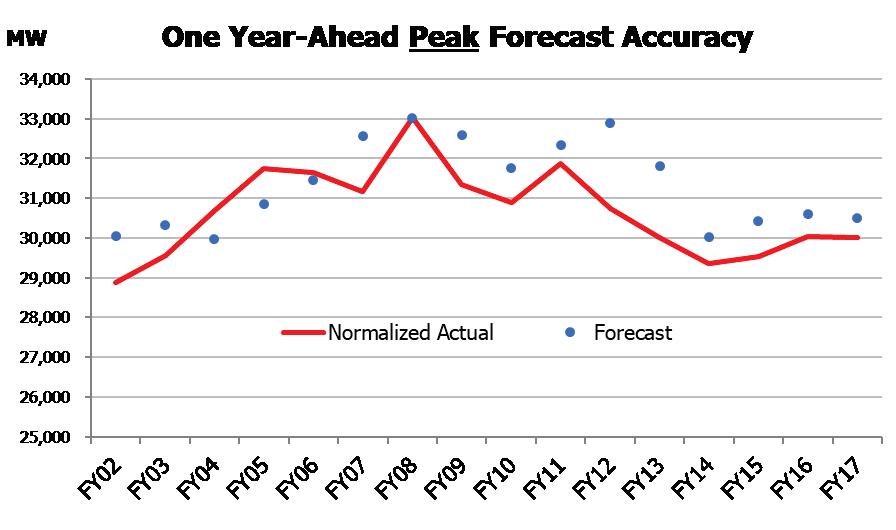
Figure 4-2 is a comparison of weather-normalized actual annual energy requirements in gigawatt-hours (GWh) to energy forecasts from one year earlier. Energy is somewhat less volatile than peaks, which are based on a single hour of each year, because energy is the
sum of all the hours of the year. This difference makes energy easier to forecast; hence, year-ahead forecast variances tend to be smaller.
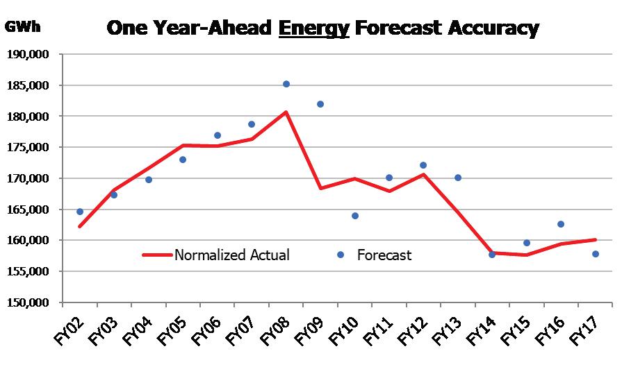
accuracy is assessed by using historical actuals for forecast variables and checking to see how close the models reproduce historic power demand. Rsquared (R2) is a statistical measure of how well the regression predictions approximate real data points. This back testing methodology indicates that TVA’s forecast model explains 98 percent of the variation, as measured by the R2, in historic demand and estimates
monthly demand within a monthly average absolute error of 1.4 percent. Fundamentally, if TVA had perfect foresight pertaining to the macro environment, the actual demand would be within +/- 1.4 percent Figure 4-3 compares the back-tested prediction (x-axis) to the actual observations (y-axis).
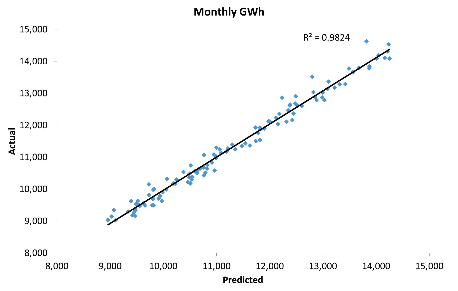
The remainder of the forecast error is caused by assumptions about market fundamentals. Forecasts of future economics, demographics and efficiency improvements drive expected demand for power. Variation in the expected business environment manifest as forecast variance. For example, at the height of the Great Recession (FY09), TVA’s weathernormalized forecast variance was 8.0 percent and 4.0 percent for System Energy and Peak, respectively, driven by the significant recession that was not part of the economic forecast. Impacts from changes in the underlying market fundamentals highlights the value in scenario analysis.
Over the next couple of decades, the Current Outlook anticipates system energy to remain flat at a 0.0 percent compound annual growth rate (CAGR) and peak demand to grow at a 0.3 percent CAGR These
forecasts are very similar to the actual growth over the FY02 through FY17 period for energy (-0.1 percent CAGR) and peak (0.3 percent CAGR) These expectations are a function of both economics and energy efficiency projections. Slower economic growth, driven by the baby boomers’ retirement, and an evertightening regulatory environment are both anticipated to moderate future energy growth.
To deal with the inherent uncertainty in forecasting, TVA uses a range of forecasts. Each forecast corresponds to different scenarios that reflect higher or lower loads compared to the Current Outlook The Current Outlook scenario for the IRP is the forecast that TVA prepared for the FY19 Long Range Financial Plan in the spring of 2018. The range of forecasts for system peak load and energy requirements in the IRP are shown in Figures 44 and 4-5, respectively. Both include the Current Outlook scenario and the highest and lowest growth scenarios that are modeled. They are the Valley Growth
scenario and the Rapid DER Adoption scenario, respectively. Annual peak load growth over the 2019 through 2038 time period is 0.3 percent in the Current Outlook scenario and varies from a -0.7 percent CAGR in the lowest peak scenario to a 1.7 percent CAGR in
the highest growth scenario System energy requirements are flat in the Current Outlook scenario with energy declining annually 1.5 percent in the lowest scenario and going as high as 2.0 percent annually in the highest growth scenario.
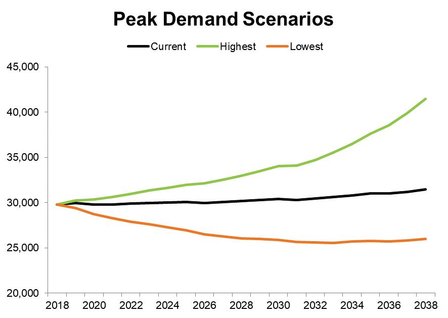

2018 - 2038
Annual Growth Rates
Highest Scenario: 1.7%
Current Outlook: 0.3%
Lowest Scenario: -0.7%
2018 - 2038
Annual Growth Rates
Highest Scenario: 2.0%
Current Outlook: 0.1%
Lowest Scenario: -1 5%
The use of ranges ensures that TVA considers a spectrum of electricity demand in its service territory and reduces the likelihood that its plans are overly dependent on a single-point estimate of demand growth. Alternative scenarios highlight the risk inherent in forecasting and planning to a single point estimate The scenario-generated ranges are used to inform planning decisions beyond pure least-cost considerations based on a specific demand in each year
To maintain reliability, power providers must always have more generating capacity available than required to meet peak demand. This additional generation, called “reserve capacity,” must be large enough to cover the loss of the largest single operating unit (contingency reserves), be able to respond to momentby-moment changes in system load (regulating reserves) and replace contingency resources should they fail (replacement reserves). Total reserves must also be sufficient to cover uncertainties such as unplanned unit outages, undelivered purchased capacity, severe weather events, or load forecasting error.
Through a recent study, TVA identified planning reserve margins for both the summer and winter peak seasons. The reserve margin study is based on a probabilistic analysis that considered the uncertainty of unit availability, transmission capability, weather-dependent unit capabilities (e.g., hydro, wind and solar), economic growth and weather variations to compute expected reliability impacts and costs. TVA selected planning reserve margins for summer and winter that targeted industry best-practice levels of reliability, while also minimizing the cost of reserves and reliability events to the customer. Based on this methodology, TVA’s
current planning reserve margin is 17 percent above peak load requirements in the summer and 25 percent above peak load requirements in the winter Additional detail about the Reserve Margin study can be found in Appendix D.
The third step in the process of analyzing future power needs is to identify the supply- and demand-side resources currently available to meet future power demand. TVA’s generation supply consists of a combination of existing TVA-owned resources; budgeted and approved projects such as new plant additions and updates to existing assets; and existing power purchase agreements (PPAs).
Generating assets can be categorized both by whether the power they produce is used to meet base, intermediate or peak demand or used for storage, and by capacity type or energy/fuel source.
Figure 4-6 illustrates the uses of baseload, intermediate and peaking assets. Although these categories are useful, the distinction between them is not always clear-cut. For example, a peaking unit, which is typically used to serve only intermittent but short-lived spikes in demand, may be called on from time to time to run continuously for a limited period even though it may be less economical to do so. This may be due to transmission or other power system constraints. Similarly, some baseload units are capable of operating at different power levels, giving them some characteristics of an intermediate or peaking unit. This IRP considered strategies that take advantage of this range of operations.
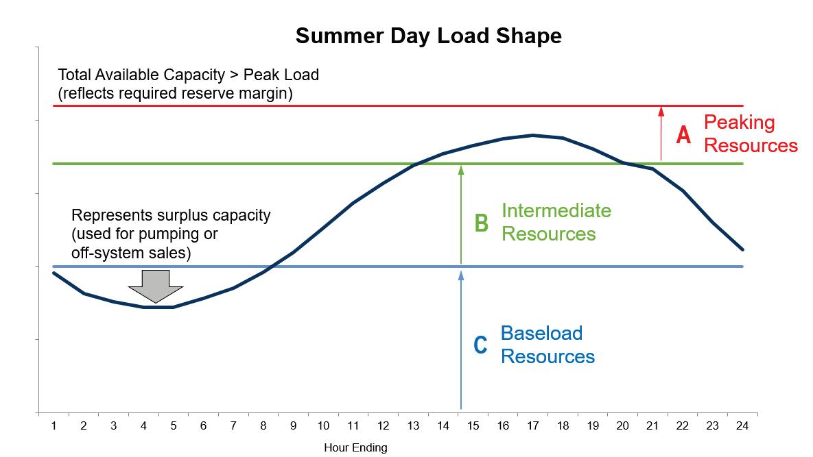
Due to their lower operating costs and high availability, baseload resources are used primarily to provide continuous, reliable power over long periods of uniform demand. Baseload resources typically have higher construction costs than other alternatives, but also have lower fuel and variable costs, especially when fixed costs are expressed on a unit basis (e.g., dollars per MWh). An example of a baseload resource is a nuclear power plant.
Some energy providers also use larger coal units and natural gas-fired combined cycle (CC) plants as incremental baseload generators. Natural gas-fired CC plants have become more attractive for baseload generation as the fundamentals of fuel supply and demand have changed and as access to shale gas has grown
Intermediate resources are used primarily to fill the gap in generation between baseload and peaking needs. They also provide backup and balance the supply of energy from intermittent wind and solar generation.
Intermediate units are required to produce more or less output as the energy demand increases and decreases over time, both during the course of a day and seasonally. Given current fuel prices and relative generating efficiencies, these units are typically more costly to operate than baseload units but less expensive than peaking units.
Intermediate generation comes from natural gas-fired CC plants and smaller coal units and also from wind and solar generation. Solar’s energy profile aligns more closely with summer load shapes and wind with winter load shapes, and the availability of energy storage technologies increases the ability to leverage these intermittent resources
Hydro generating assets can generally be categorized as intermediate resources, but their flexibility allows them to operate the full range from baseload to peaking. The limitation of hydro generation is restricted more by water availability and the various needs of the river system such as navigation, flood control and recreation.
Peaking units are expected to operate infrequently during short-duration, high demand periods. They are essential for maintaining system reliability requirements, as they can start up quickly to meet sudden changes in either demand or supply. Typical peaking resources are natural gas-fired frame combustion turbines (CTs), aeroderivative CTs, reciprocating internal combustion engines (RICE), and conventional hydro generation
Storage units usually serve the same power supply function as peaking units but use low-cost, off-peak electricity to store energy for generation at peak times. An example of a storage unit is a hydro pumpedstorage plant. These plants pump water to a reservoir during periods of low demand and release it to generate electricity during periods of high demand. Consequently, a storage unit is both a power supply source and an electricity user. Lithium-ion batteries are another example of a storage resource.
Power system peaks are measured in terms of capacity, the instantaneous maximum amount of energy that can be supplied by a generating plant and collectively by the power system.
For long-term planning purposes, capacity can be defined in several ways:
• Nameplate capacity is the theoretical design value or intended maximum megawatt output of a generator at the time of installation.
• C apability is the maximum dependable loadcarrying ability of units or the number of megawatts that can be delivered by a generating unit without restrictions (i.e., does not reflect temporary capacity restrictions caused by known fuel or mechanical derates) and less station power
• N et dependable capacity is the maximum dependable output less all known adjustments (e.g., transmission restrictions, station service needs and fuel derates) and is dependent on the season. This value, which is used by
capacity planners, is typically determined by performance testing during the respective season. TVA uses both summer and winter net dependable capacities of units in the analysis, given the dual-peaking nature of the system.
Overall power system production is measured in terms of energy (i.e., megawatt-hour). Energy is the total amount of power that an asset delivers in a specified time frame. For example, one MW of power delivered for one hour equals one megawatt-hour (MWh) of energy.
The capacity factor of a power plant is a measure of the actual energy delivered by a generator compared to the maximum amount it could have produced at the nameplate capacity. Assets that run constantly, such as nuclear plants, provide a significant amount of energy with capacity factors greater than 90 percent.
Assets that are used infrequently, such as a combustion turbine, provide relatively little energy with capacity factors of typically less than five percent, although the energy they produce is crucial since it is often delivered at peak times.
Variable energy resources such as solar and wind have capacity factors based on their shapes, or pattern of generation across the days and seasons. Utility-scale solar capacity factors can approach 25 percent, and wind capacity factors from Midwest farms average around 40 percent. Capacity factors for these resources vary by location For example, solar capacity factors in very sunny regions of the U.S. are higher than in less sunny regions, and wind farms in the Midwest plains have higher capacity factors than in-Valley installations.
High capacity factor unit:
A 1 , 200 - MW nuclear unit could theoretically produce 10,510 GWh of energy if it ran every hour of the year. After planned annual outages, the unit will typically produce 9,460 GWh or 90 percent of its theoretical capacity.
Low capacity factor unit:
A 250 - MW natural gas- fired combustion turbine (CT) unit could theoretically produce 2,190 GWh of energy if it ran every hour of the year. However, CT units generally have a capacity factor less than 5 percent, w hich means the unit would likely operate about 440 hours of the year and produce about 110 GWh.
Energy efficiency also can be measured in terms of capacity and energy. Even though energy efficiency does not input power into the system, the effect is similar because it represents power that is not required from another resource. Demand response also is measured in capacity and energy. However, unlike energy efficiency, it does not offer a significant reduction in total energy used.
TVA uses a wide range of technologies to meet the needs of the Valley residents, businesses and industries. Figure 4-7 shows the current projection for capacity demand and for capacity supply from existing resources and power purchase agreements, highlighting the capacity gap. Applying the Base Case strategy, TVA then uses the planning model to optimize the resource portfolio to fill this gap while scheduling the contribution of current energy efficiency, demand response, and renewable programs and considering
retirements where economic The optimized result for the Base Case strategy evaluated in the Current Outlook scenario is shown later in the results section of this document
Figure 4-7 includes both owned and purchased resources, in megawatts of summer net dependable capacity, and is divided into fuel-type (i.e., nuclear, hydro, coal). The chart builds up from the bottom generally in a baseload, intermediate and peaking order, as some assets can serve dual roles.
Figure 4-7 shows how TVA’s existing capacity portfolio is expected to change through 2038. This projection serves as the baseline firm capacity for optimizing all portfolios. The existing assets only include resources that currently exist; assets that are under contract; TVA Board-approved changes to existing resources such as refurbishment projects; and TVA Board-approved additions. Existing resources decrease through 2038 primarily because of the retirement of coal-fired units and the expiration of existing contracts (power purchase agreements). The renewable component of the existing portfolio is primarily composed of wind PPAs that expire in the early 2030s. Because the power generated from wind and other renewable resources is intermittent, the firm capacity (or the amount of capacity that can be applied to firm requirements) for these assets is lower than the nameplate capacity. Figure 4-8 identifies expiring and retiring resources that are currently on the TVA system and their respective capacities
Having a diverse portfolio of resource types – coal, nuclear, hydro, natural gas and renewable resources –and being able to use these resources in different ways enables TVA to provide reliable, low-cost power while minimizing the risk of disproportionate reliance on any one type of resource.
Approximately 36 percent of TVA’s capacity is currently sourced from emission-free assets such as nuclear power, renewable resources including hydro, and interruptible load management. The renewable category shown throughout this document is based on
Existing CT/Diesel
Existing EEDR
Existing Renewables
Existing CC
Existing Coal
Existing PS Hydro
Existing Hydro
Existing Nuclear
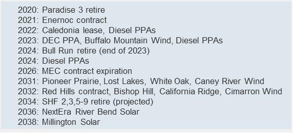
modeled outputs of energy from renewable sources such as wind, solar, and biomass. This metric is not intended to represent a quantity of certified renewable energy credits.
In FY18, 39 percent of TVA’s energy was produced from the nuclear fleet. Coal plants produced about 21 percent of the generation, while the gas fleet produced about 26 percent. Hydro plants produced approximately 10 percent, and 3 percent was produced from wind and solar sources. The remaining one percent results from TVA programmatic energy efficiency efforts, which have been reduced due to increasingly effective USDOE codes and standards
As noted previously, a capacity gap is the difference between total supply and total demand. More
specifically, it is the difference in megawatts between a power provider’s existing firm capacity and the forecast annual peak adjusted for any interruptible customer loads and long-term planning reserve requirements (i.e., (i.e., 17 percent for summer and 25 percent for winter).
Figure 4-9 shows TVA’s estimated capacity gap or shortfall based on the existing firm capacity and the annual firm requirement for the Current Outlook scenario for the summer and winter peaks The aim of the IRP is to evaluate strategies and portfolios to meet the capacity gap across a wide range of potential future scenarios.
TVA also considers the capacity gaps that might occur within the other scenarios. Figure 4-10 shows the range of capacity gaps corresponding to all the scenarios, ranging from the Valley Load Growth scenario on the high end to the Rapid DER Adoption scenario on the low end All scenarios are described in detail in Chapter 6
When optimizing the portfolio, power system analysis evaluates the most economical way to meet the capacity gap and associated energy needs, considering resource options and promotions applicable in each strategy.
Maintaining the diversity of energy resources is fundamental to TVA’s ability to provide low-cost, reliable and clean electric power to Valley residents, businesses and industries. For this reason, TVA considered the addition of a wide range of supply-side generating resources, as well as energy efficiency and other demand-side resource options, to fill the forecasted 20year capacity and energy gaps identified through the power needs analysis described in Chapter 4.
The power needs analysis indicates that, under the Current Outlook scenario, TVA will require additional capacity and energy of about 1,200 MW and 7,100 GWh by 2028, growing to about 4,400 MW and 13,800 GWh by 2038.
During the scoping process, TVA identified a broad range of energy resources that could be used to fill the predic ted capacity and energy gaps. The next two sections explain the criteria that were used to reduce this list to a manageable portfolio of expansion options. For a complete list of resource options considered, see Chapter 5, Energy Resource Options, of the a ssociated EIS
Two criteria were used to ensure that only viable energy resource options were considered in the IRP analysis. To be considered, resource options must:
• Use a proven technology, or one that has reasonable prospects of becoming commercially available in the planning horizon
• Be available to TVA within the region or be available to be imported through market purchases.
Technology is a key factor in TVA’s ability to fulfill its mission in a balanced way. TVA continues to pursue technological advances to become more efficient and sustainable. As part of its mission under the TVA Act, the agency is called upon to be a leader in technology innovation.
In the 2015 IRP, DER was included in the load forecast as a load modifier that reduced demand for electricity from TVA, and energy efficiency and demand response were modeled as selectable resources. In the 2019 IRP, TVA has made further refinements in modeling behind-the-meter generation in the load forecast, including variations across the scenarios. We have also modeled distributed generation resources, including combined heat and power, and distributed solar and storage. There are targeted levels of adoption of these distributed resources based on incentive levels in each strategy. Further information on how these resources were modeled is included in Appendices A, B and C.
To compare energy resource options available for new generation objectively, it is important to have consistent data regarding the cost and operating characteristics of each option. A list of characteristics used in the 2019 IRP are identified and defined in Table 5-1 and Table 5-2. Section 5.2.2 provides the numerical values for some of these parameters for the new assets.
Unit capital costs
Capital escalation rates
Construction spend schedule
Fixed operating and maintenance costs (FOM)
Variable operating and maintenance costs (VOM)
Fuel expenses
Each technology type must have a representative $/kW unit, which is considered a total installed cost. Total installed cost includes equipment, engineering and interest during construction in present day dollars.
Since capital costs typically increase over time, TVA assumes that capital costs escalate at the forecast rate of inflation for most resources. However, some energy technologies (e.g. solar and battery storage) are rapidly evolving, so TVA assumes declining costs for these resources.
Some technologies take a long time to build. Construction times for nuclear units, for example, average about 10 years. To estimate the cash flow for the construction of a long-lead time build unit such as a nuclear unit, the percent of total capital dollars spent in each year is required. This metric is typically not needed for renewable assets which are smaller in scale and generally built in less than a year.
FOM costs are independent of the number of hours of operation or amount of electricity produced and are generally expressed in dollar per kilowatt per year ($/kW-yr). FOM includes operating and maintenance labor, plant support equipment, administrative expenses and fees required by regulatory bodies.
VOM costs are dependent on the number of hours of operation and are generally expressed as a dollar per megawatt-hour ($/MWh). VOM costs include consumables like raw water, waste and water disposal expenses, and chemicals and reagents. VOM costs do not include fuel expenses.
Fuel is the material that is consumed to generate electricity – for example, coal, natural gas, uranium and biomass. These costs are typically expressed in dollar per million British thermal units ($/mmBtu) and include the delivery charges.
Transmission A new generating resource has to be connected to the transmission system. Costs are typically expressed in a dollar per kilowatt ($/kilowatt) unit
Integration cost Intermittent resources require the balance of system resources to absorb sub-hourly fluctuations, driving an integration cost. Further details on the cost study are included in Appendix D. New solar and wind resources have integration costs, expressed in $/MWh.
Flexibility benefit
Capacity credit
Full load heat rate
Highly flexible resources provide a sub-hourly benefit associated with ability to more efficiently absorb subhourly fluctuations in intermittent resources. Further details on the benefit study are included in Appendix D. New aeroderivative CTs and utility battery storage resources have flexibility benefits, expressed in $/kW.
Each unit must have a summer and winter net dependable capacity rating in megawatts.
The capacity credit is the amount of capacity immediately available at the highest demand times. The capacity credit must be estimated for variable units or non-dispatchable resources.
A heat rate must be specified for each unit for summer and winter. A heat rate is a measure of the consumption of fuel necessary for a unit to produce electricity. Heat rates are expressed in British thermal units per kilowatt hour (Btu/kWh) and are based on a full-load heat rate. Heat rates are considered longterm planning assumptions and include the expected degradation in the heat rate of a unit after the first two years. Although a heat rate is not typically associated with a nuclear unit, one is necessary to model the fuel costs.
Unit availability A date when each unit would be available for operation must be specified. Unit availability is restricted by technical feasibility or commercial availability, as well as permitting and construction times. For example, if it takes five years to build a combined cycle plant, then a new CC could not be selected prior to five years into the planning horizon.
Book life
The book life of a unit is the number of years a resource is expected to be in service for accounting purposes. Book life is the financial payback period which represents the amount of time the asset is expected to be used and useful. A license extension, beyond the original asset life, is not assumed with any new generating option.
TVA’s existing assets, budgeted and approved projects, and power purchase agreements are considered as the baseline firm capacity in the IRP evaluation. These assets are generally expected to continue operating through the duration of the planning period or through the terms of existing power purchase agreements and other contracts, where applicable.
Options to meet the forecast net system requirements identified in Chapter 4 include:
• Building new generating units
• Entering into new power purchase agreements
• Developing energy efficiency and demand response programs
• Retiring existing resources
The next two sections describe existing and potential new generation by resource category, as well as retirement options. For a comprehensive description of all resource option attributes, characteristics and technologies, see Chapter 5, Energy Resource Options, of the associated EIS
TVA currently operates seven nuclear reactors: three at Browns Ferry Nuclear Plant, two at Sequoyah Nuclear Plant and two at Watts Bar Nuclear Plant. These plants have a combined generating capacity of about 7,700 MW. Extended power uprates for the three Browns Ferry units have been approved by the TVA Board and will be completed by the end of 2019. These uprates will add about 450 MW of additional capacity at the Browns Ferry plant.
The three units at Browns Ferry Nuclear Plant have license expiration dates of 2033, 2034, and 2036, respectively. TVA will evaluate non-renewal of these licenses in the No Nuclear Extensions scenario, where
no nuclear units in the U.S. will be allowed to operate beyond 60 years. All other scenarios assume that TVA is granted a Second License Renewal (SLR) by the Nuclear Regulatory Commission (NRC). The two units at Sequoyah are licensed for operation through 2040 and 2041, respectively. Watts Bar Unit 1 is licensed for operation through 2035 (initial 40 year license), and Watts Bar 2 began commercial operation in October 2016.
5.2.1.2 Coal
TVA operates six coal-fired power plants consisting of 26 active generating units with a total capability of almost 7,900 MW TVA uses a value lower than the capability of a resource, based on its summer and winter net dependable capacity Table 5-3 is a snapshot of the planning assumptions for the coal units, including the forecasted retirement of the uncontrolled Shawnee units in 2034 to meet air quality standards. Following detailed evaluation, on February 14, 2019, the TVA Board of Directors voted to retire Paradise Unit 3 by the end of 2020 and Bull Run by the end of 2023. All cases reflect retirements of these units in 2020 and 2023, respectfully.
In addition to TVA-owned coal-fired units, TVA has access to the output from a coal-fired power plant with a generating capacity of about 440 MW through a long-term power purchase agreement that expires in 2032.
TVA operates 87 natural gas-fired combustion turbines (CT) at nine power plants with a combined generating capability of about 5,700 MW and 14 combined cycle (CC) units at eight plants with approximately 6,800 MW of capability. TVA has power purchase agreements for about 1,300 MW of capability from two merchant combined cycle gas plants, with agreements expiring in the early to mid-2020s.
TVA currently owns five diesel generators with a total capability of 9 MW.
Allen
Bull
Colbert
Cumberland 2
Gallatin 4
John Sevier 4
Johnsonville 10
Kingston 9
Paradise
Shawnee
TVA operates 109 conventional hydro generating units at 29 dams. These units have the capability to generate about 3,800 MW of electricity. All IRP portfolios reflect investing in and maintaining TVA's existing hydroelectric fleet. TVA has completed 60 hydro unit modernization projects out of 109 conventional hydro units. TVA plans to modernize two to three units per year, and the program is perpetual in nature to maintain capacity over time.
In addition, TVA has a long-term power purchase agreement with the U.S. Army Corps of Engineers for eight dams on the Cumberland River system. These facilities provide about 400 MW of capability
TVA anticipates about 70 percent of this hydro capability to be available at the summer peak hour, given the operational constraints of the hydro units.
TVA operates one large energy storage facility. The Raccoon Mountain Pumped-Storage Plant has four generating units with a Summer Net Dependable (SND) capacity of about 1,600 MW Raccoon Mountain is TVA’s largest hydro facility and provides critical flexibility
Continue to operate
Continue to operate
Continue to operate
to the TVA system by storing water at off-peak times for use when demand is high.
TVA purchases all of the power produced by the Buffalo Mountain wind farm in Anderson County, Tennessee. Buffalo Mountain is one of the largest wind farms in the Southeast, with 15 turbines and 27 MW of nameplate capacity. As defined in section 4.3.2, the nameplate capacity is the maximum technical output of a generator, or the theoretical design value.
TVA has long-term power purchase contracts with seven wind farms located in Illinois, Kansas and Iowa. These facilities provide about 1,200 MW of nameplate capacity. TVA anticipates about 14 percent and 31 percent of the nameplate to be available for peak summer and winter requirements, respectively These agreements expire in the early 2030s. TVA obtains the renewable energy credits from these farms. Renewable energy credits are a separate commodity formed from the production of energy at designated sites.
TVA owns 14 photovoltaic (PV) installations with a summer capability of approximately 1 MW. TVA also purchases solar power through several programs and
long-term power contracts totaling 370 MW of nameplate capacity with about 250 MW expected to be available at the summer peak hour. TVA obtains the renewable energy credits from these sites, and the existing PPAs extend through the late 2030s. Solar power purchase agreements signed subsequent to the spring of 2018 when baseline firm capacity was established for this IRP are not included in existing assets. This includes agreements signed for about 700 MW of solar nameplate capacity to meet specific customer needs.
TVA purchases about 50 MW of biomass-fueled generation through existing programs.
TVA’s energy efficiency portfolio focuses on reduction in peak demand and energy savings. From FY07-FY18, these efforts contributed about 400 MW of summer peak demand reduction and saved about 2450 GWh of energy annually. These savings are adjusted for applicable transmission and distribution (T&D) losses, free rider/driver discounts, realization rates, and performance adjustments for actual weather.
Demand response programs focus on reduction of peak demand. Under these programs, TVA direct-
served customers and local power companies can reduce their power bills by allowing TVA to suspend availability of power in the event of a power system, economic, or reliability need. These programs provide about 1800 MWs of peak reduction.
A complete list of viable new resource options for evaluation in this IRP is provided below. All options are based on a generic location and unit availability rounded to the next full year A detailed discussion by resource category follows.
With a focus on DERs in this IRP, TVA also leveraged input from the Distributed Generation Information Exchange (DGIX) to inform resource characteristics and costs. DGIX input specifically helped inform inputs for distributed solar and storage, CHP, and electric vehicles.
An independent third-party reviewed and compared the parameters to proprietary and other industry sources to ensure the modeled unit characteristics and assumptions were representative of the respective generating technologies. See Appendix A for the letter summary of the benchmarking efforts of Navigant Consulting, Inc. as well as a brief discussion of TVA’s internal benchmarking on resource costs ($/kW).
Nuclear
• Pressurized Water Reactor (PWR)
• Advanced Pressurized Water Reactor (APWR)
• Small Modular Reactor (SMR)
Coal
• Supercritical Pulverized Coal 1x8
• Supercritical Pulverized Coal 2x8
• Integrated Gasification Combined Cycle (IGCC)
• Integrated Gasification Combined Cycle with Carbon Capture and Storage (IGCC CCS)
• Supercritical Pulverized Coal 1x8 with Carbon Capture and Storage
• Supercritical Pulverized Coal 2x8 with Carbon Capture and Storage
Natural Gas
• Combustion Turbine 6x (LMS 100)
• Combustion Turbine 4x (LMS 100)
• Combustion Turbine 2x (LMS 100)
• Combustion Turbine 3x (7FA)
• Combustion Turbine 4x (7FA)
• Combined Cycle 1x1
• Combined Cycle 2x1
• Combined Cycle 3x1
• Combined Cycle Supplemental Duct-firing (1x1, 2x1, 3x1)
• Combined Cycle With Carbon Capture and Storage
• Reciprocating Internal Combustion Engine (RICE) 12x
• Reciprocating Internal Combustion Engine (RICE) 6x
• Reciprocating Internal Combustion Engine (RICE) 2x
• Commercial & Industrial Combined Heat and Power (CHP)
Hydroelectric
• Hydro Spill Addition
• Hydro Space Addition
• Hydro Run of River
Energy Storage
• Pumped Storage
• Utility Battery Storage
• Residential Battery Storage
• Compressed Air Energy Storage (CAES)
• Fuel Cells
• Advanced Chemistry Battery
There are three nuclear expansion options available to fill the expected capacity gap: a Pressurized Water Reactor (PWR), an Advanced Pressurized Water Reactor (APWR) and a Small Modular Reactor (SMR).
SMRs are a new type of nuclear reactor in which the components are manufactured in a factory and then assembled together onsite. T he individual units are smaller in size, allowing for increased flexibility in installation and use. New units could be located at existing nuclear plants or at other sites beneficial to the transmission system or local resiliency.
Wind
• Midcontinent Independent System Operator (MISO)
• Southwest Power Pool (SPP)
• In-Valley
• High Voltage Direct Current (HVDC)
Solar
• Utility -scale Single-axis Tracking
• Utility -scale Fixed-Axis
• Large Commercial-scale
• Small Commercial-scale
• Residential Scale
Biomass
• New Direct Combustion Biomass
• Repowering Existing Coal with Biomass
Energy Efficiency
• Residential
• Commercial
• Industrial Demand Response Electrification
Retirement Options
• Gas Combustion Turbines > 40 years old (as early as 2020)
• Uncontrolled Shawnee units (as early as 2020)
• All Other Coal Units (as early as 2025)
• Browns Ferry Nuclear Units 1-3 (as early as 2033)
As mentioned previously in Chapter 4, the retirement of the three Browns Ferry units is being evaluated in the No Nuclear Extensions scenario. In this scenario, it was mentioned there could be subsidies to drive small modular reactor technology advancements and improved economics. What is contemplated is more about demonstrating modular construction processes efficiently in a nuclear application, in order to reduce cost and schedule uncertainties for subsequent SMR facilities. Strategy C, which emphasizes small, agile resources, includes two SMRs totaling 1,200 MW forced in to replace one of three Browns Ferry units.
Table 5-4 shows some of operating characteristics used to model each option. Summer net dependable capacity, summer full load heat rate, unit availability and
book life are explained earlier in this section The annual outage rate percentage includes forced and planned outages. See Chapter 4, Section 4.3.2, for a discussion of the different types of capacity ratings.
The 2019 IRP includes six coal expansion options, including two integrated gas combined cycle (IGCC) options and four supercritical pulverized coal (SCPC) options as shown in Table 5-5.
IGCC technology converts coal into gas. One IGCC option has carbon capture and sequestration (CCS) and one does not. The CCS technology option is assumed to be commercially available starting in 2028 and has a 90 percent carbon dioxide (CO2) capture rate. Coal units typically have a CO2 emission rate of 205 pounds per million BTUs of coal burned; therefore, the CCS technology would reduce the CO2 rate to 20.5 pounds per million BTUs of coal burned. The modeled CO2 emissions incur an emission penalty in the form of a dollar per ton of CO2 emitted.
Two of the four SCPC options have one steam generator with a supercritical steam cycle. One of these options includes CCS technology; the other does not. The other two SCPC options have two steam generators with supercritical steam cycles. Again, one of these options includes CCS technology, and one does not.
In addition to the approved retirements of Paradise Unit 3 in 2020 and Bull Run in 2023, there are several additional coal retirement options available for model selection:
• Uncontrolled Shawnee Units (2,3,5-9) as early as 2020
• All other coal units as early as 2025
The IRP evaluation includes three reciprocating internal combustion engine (RICE) options, five simple cycle combustion turbine (CT) options, and four combined cycle (CC) natural gas fueled options. The RICE engines are available in packages of two, six, or twelve engines. The simple cycle frame CTs are available with either three or four turbines The other three CT options are aeroderivatives in packages of two, four, or six turbines as shown in Table 5-6
The CC options have one turbine and one steam generator (CC 1 by 1), two turbines and one steam generator (CC 2 by 1), or three turbines and one steam generator (CC 3 by 1). CC units have supplemental capacity termed duct-firing capacity that adds approximately 100 MW to the base capacity shown. The fourth CC option is a 3 by 1 integrated gasification combined cycle (IGCC) with carbon capture and storage (CCS). The CO2 emission rate for a typical gas unit is 117 pounds of CO2 per million Btus of gas burned. The modeled gas units incur emission charges based on a dollar-per-ton emission penalty for those scenarios with a CO2 penalty
In addition to options for TVA to build gas-fueled units, the IRP evaluation includes options for continuing to
purchase power from existing merchant gas plants or acquiring those plants PPAs are available for selection based on competitive information which cannot be disclosed. PPA options are evaluated similar to build options with a few slight differences. One difference is that when present value revenue requirements resulting from the expansion model selections are converted into cash flows, then the build options have significant capital expenditures that match the construction spend schedule (noted in section 5.1.2) versus the PPA options which have levelized cash flow payments based on the terms of the contract (similar to a mortgage). The other difference for PPAs is that if the asset is located outside of the TVA transmission area, then the necessary transmission wheeling charges are included.
Combined heat and power (CHP), a distributed gas resource, is offered as an option. Rather than being selectable, various levels of CHP adoption are included to represent consumer response to incentive levels applicable in each strategy, as described in Appendix F.
In addition, there are options for retirement of TVA’s older simple cycle frame CTs as early as 2020.
TVA expects to phase out petroleum power purchases by 2028. There are no diesel fuels or other petroleumbased resource options as a primary fuel source under consideration in the IRP because of emissions from these facilities.
Two new hydro projects are included in the IRP evaluation. They include adding additional hydro turbines to existing dam facilities where there is space available with structural modifications. The other project would add turbines at existing dam facilities where water that is now spilled could be used to power more turbines.
Both projects are similar to the larger TVA hydro system and are energy-limited units. Energy-limited units are resources that cannot be dispatched (in the
model) based on price ($/MWh) as are traditional thermal generating resources, such as nuclear, coal and gas. Hydropower cannot be dispatched based on price alone because water releases in the Tennessee River system also are required for municipal and industrial uses, navigation, flood damage reduction, recreation, water quality and other purposes. For this reason, TVA includes a fixed amount of monthly energy in the model for conventional hydro stations. The model then uses the hydro energy to level the load shape served by other stations.
Since hydro plants do not use fuel, a heat rate is not needed for modeling.
Small- and low-head hydropower, called run of river, also is included as an IRP resource option. The hydro expansion options are shown in Table 5-7.
The IRP evaluation includes a new hydro pumpedstorage unit as a resource option The pumped-storage option would use three reversible turbine generators to either take electricity from the grid by pumping water into a higher altitude reservoir during periods of excess power or add electricity to the grid by using the pumped water to power a turbine as it falls from the upper to the lower reservoir.
A compressed air energy storage (CAES) option also is included. A CAES plant is similar to a pumped-storage plant but, instead of pumping water from a lower to an upper reservoir, a gas turbine is used to compress air often into an underground cavern where it can be stored under pressure until electricity is required. The pressurized air is then heated and directed through a conventional generator to produce electricity.
Battery storage is included as an option at the utility scale and the residential scale Rather than being selectable, distributed storage is modeled at various levels of adoption to represent consumer response to incentive levels applicable in each strategy, as described in Appendix F. TVA is also including fuel cells and advanced chemistry batteries as options in this IRP The storage options are shown in Table 5-8
Storage efficiency is included in modeling all these energy storage options because of the energy losses inherent to the energy conversion process and due to the loss of water or air during storage. The storage efficiency percentage for these energy storage options represents the efficiency of one cycle (i.e., pumping water, then releasing).
Because TVA cannot take direct advantage of the tax credits and other investment incentives offered by the federal government to encourage wind power development, it has been more financially advantageous to acquire wind power resources through PPAs. This approach allows TVA to include wind as a resource option in the IRP. The purchase of wind resources as a PPA, whether produced in or imported to the TVA region, lowers the costs of these resources to TVA and its customers. TVA may evaluate the option of building wind facilities in the future if investment incentives and/or future federal or state renewable mandates change.
Four wind options are included in the IRP evaluation as shown in Table 5-9 The Midcontinent Independent System Operator (MISO), the Southwest Power Pool (SPP) and the In-Valley options represent various wind resources in different regional transmission areas. The High Voltage Direct Current (HVDC) option would use a direct current (DC) bulk transmission system. The HVDC transmission system would reduce power losses that are typical of the more common alternating current (AC) transmission systems. The HVDC option would require a third-party to permit and build a new transmission line, driving a later availability date than the other options.
Wind resources are energy- and capacity-limited resources. For this reason, TVA uses an energy production profile to dispatch wind energy rather than price. The method used for wind resources is somewhat similar to hydro resources except that an hourly generation schedule (not a monthly amount) is pre-loaded into the capacity expansion model. TVA also applies a capacity credit since the total nameplate capacity of a wind turbine cannot be expected at the time of the system peak. To determine the capacity
credit, TVA used historical data to estimate the typical wind power output at the time of the peak power demand on the TVA system. This resulted in a 14 percent capacity credit, meaning that 14 percent of nameplate capacity is expected to be available at the system summer peak. This reduced capacity is considered the summer net dependable capacity. Appendix A includes a more detailed discussion about the determination of the data assumptions for the modeling of the wind options included in this IRP
Similar to new wind generation, TVA cannot take direct advantage of the current investment incentives offered to promote solar power development, making it more financially advantageous to acquire solar power resources through PPAs. TVA may evaluate the option of building solar facilities in the future if investment incentives and/or federal or state renewable mandates change.
Five solar options are included in the IRP evaluation as shown in Table 5-10 All capacities are stated in AC terms. The utility tracking option is a single-axis tracker that allows the solar panels to follow the sun. The utility fixed option represents ground mounted fixed-axis/fixedtilt solar installations. Distributed solar options are offered at large commercial, small commercial, and residential scales. Rather than being selectable, various levels of
distributed solar adoption are included to represent consumer response to incentive levels applicable in each strategy, as described in Appendix F.
Like wind resources, solar resources are energy-limited and therefore dispatched in the model using an hourly energy production profile to ensure that solar generation is not utilized by the model when the sun is not available. Solar resources also are similar to the capacity-limited wind resources where the availability of the unit at the time of the TVA system peak is less than the full nameplate capacity. TVA applied a 68 percent capacity credit for the utility tracking unit and a 50 percent capacity credit for the fixed axis options. The unit availability date was rounded to the first full year. More details about the assumptions used in the development of the unit characteristics for these solar options can be found in Appendix A.
Two biomass options are included in the IRP evaluation as shown in Table 5-11: a new direct combustion biomass facility and a repower option, which is the
Demand response programs enable participating customers to reduce their power costs by allowing TVA to limit their power during peak demand times. These programs were modeled in the 2019 IRP, as shown in Table 5-12, based on unit characteristics similar to those used for natural gas CTs. Demand response programs are operated much like CTs, or peaking units, and focus on reduction of peak demand. However, the terms of the demand response customer
conversion of existing coal-fired units to biomass-fired units. Because biomass co-firing is considered a fuel switch opportunity, it was not included as a capacity expansion option
contracts are shorter than the expected book life of a CT unit. In all strategies, TVA assumed that current interruptible pricing products and third-party aggregation of small commercial and industrial demand response will continue with current program size limitations at the carrying cost of a CT. Also included are residential demand response expansion options for space conditioning and water heating, available beginning in 2020
The 2019 IRP builds on the innovative modeling approach used in the 2015 IRP to evaluate EE as a supply-side resource, with characteristics and costs structured similarly to conventional generating resources or power plants. More details about this modeling approach can be found in Appendix D.
This IRP includes EE programs for residential (Res), commercial (Com) and industrial (Ind) sectors as shown
in Table 5-13 Each was divided into tiers, representing distinct price points The 2019 IRP includes low-income residential EE programs, which are designed to facilitate EE improvements for those least able to afford them. The costs for these programs vary by strategy, but are enforced as required resources at the incentive level dictated by the strategy goals. For all programs, all tiers are available beginning in 2020 These programs are energy limited, similar to hydro, wind and solar units, and use annual hourly production profiles.
5.2.2.12 Electrification
Electrification is the increased adoption of electric enduse technologies displacing other commercial energy forms. Promotion of smart energy technologies with a favorable load shape should decrease carbon emissions and increase profitability for Valley businesses. While electrification is not a “resource” like the others described in this section, potential electrification offerings for the residential, commercial and industrial sectors are included as selectable
options in this IRP. The residential electrification programs focus on retrofit and new construction markets, while commercial and industrial programs focus on diverse technology offerings to help shape load. These options are also offered in three tiers at distinct price points as shown in Electrification
Expansion Options Table 5-14
This chapter describes the process TVA used to identify a target power supply mix that was based on the analysis done in the IRP. The process involves choosing the types of resources that TVA could use to meet the future power needs of its customers, recognizing that the future is uncertain and the choices need to provide flexibility to adapt. The approach tests several options around resource choices TVA could make (called strategies) in different sets of uncertain future conditions (called scenarios). The set of resource choices selected in any one future defines how TVA
would provide power to its customers under those conditions; TVA calls that set of resource choices a portfolio, and it is created by modeling a strategy in a particular scenario. These portfolios are then evaluated using key factors (called metrics) that allow TVA to capture cost, risk, environmental footprint and other aspects that should be considered when deciding the best target power supply mix.
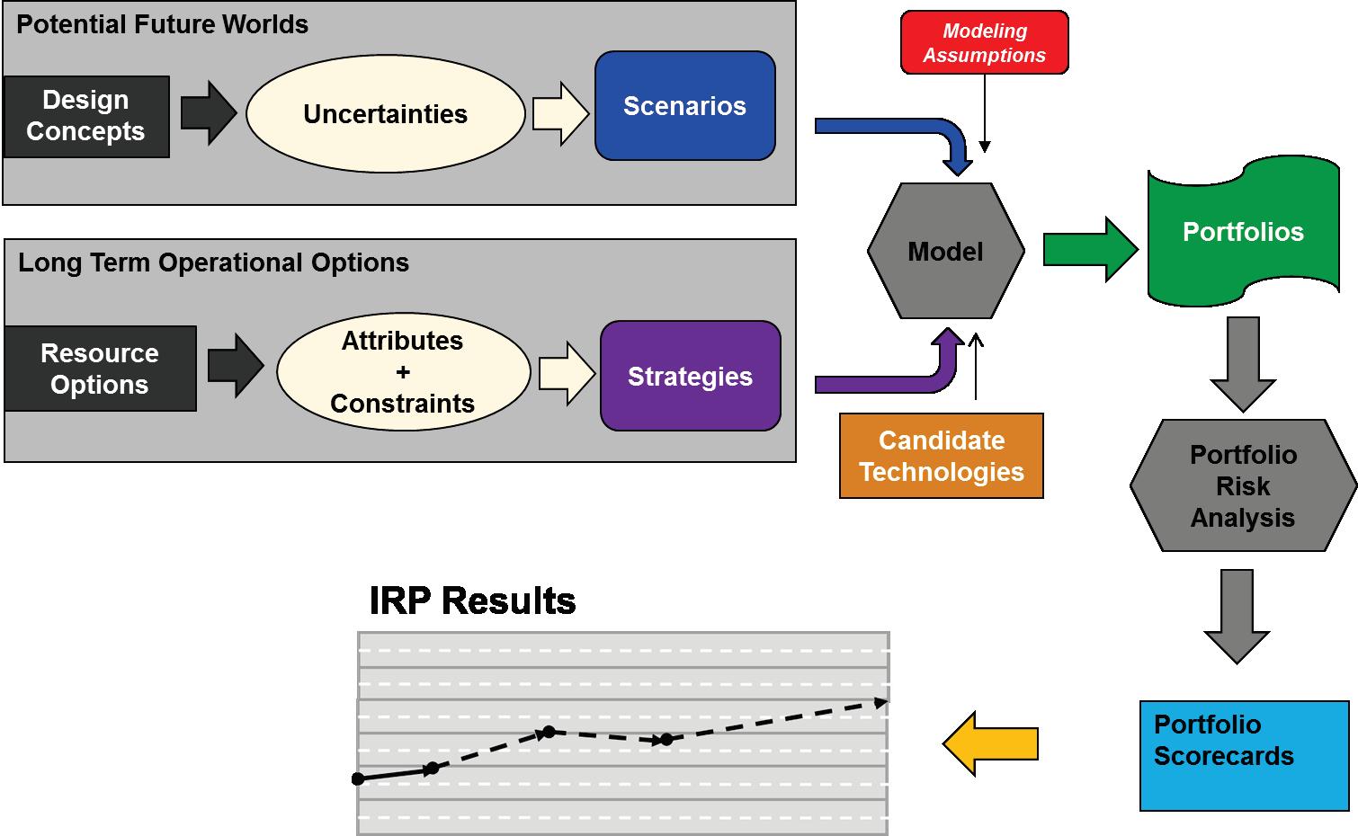
TVA uses a scenario planning approach in integrated resource planning, a common approach in the utility industry. Scenario planning is useful for determining how various business decisions will perform in an uncertain future. The goal is to develop a least-cost strategy that is consistent with TVA’s legislatively mandated mission and also delivers rate stability to its customers over a variety of future environments
Multiple strategies, which represent business decisions that TVA can control, are modeled against multiple scenarios, which represent uncertain futures outside of TVA’s control. The intersection of a single strategy and
The result of a strategy evaluated in a scenario
How uncertainty impacts the portfolio results
Standard metrics to compare portfolios
a single scenario results in a resource portfolio. A portfolio is a 20-year capacity plan that is unique to that strategy and scenario combination
While most quantitative models used in long-range planning focus on what is statistically likely based on history, market data and projected future patterns, TVA uses scenario analysis that allows for the possibility that the future could evolve along paths not suggested solely by historical trends.
The scenarios used in the IRP analysis were developed during the scoping phase of the study in 2018 The process used to develop these scenarios is described below.
The first step in developing scenarios was to work with the individuals on the IRP Working Group to identify key uncertainties. Uncertainties are factors that are likely to change in the future, affecting economics, demand for electricity, commodity prices, etc. While TVA can forecast future values for these uncertainties, they are
Uncertainty Description
Electricity Demand
Market Power Price
Natural Gas Prices
Coal Prices
Solar Prices
Storage Prices
Regulations
CO2 Regulation/Price
Distributed Generation Penetration
National Energy Efficiency (EE) Adoption
Electrification
Economic Outlook (National/Regional)
difficult to predict. The goal of scenario analysis is to study broad variations in uncertainties to cover a wide range of potential futures. The 12 uncertainties, shown in Table 6-1, were used as building blocks to construct scenarios.
These uncertainties address a range of economic, financial, regulatory and legislative conditions, as well as social trends and adoption of newer technologies. The 12 uncertainties used in defining each scenario are described in Table 6-1
The customer energy requirements (in gigawatt hours) for the TVA service territory (including losses), representing the load to be served by TVA
The hourly price of energy ($/megawatt hour) at the TVA boundary, used as a proxy for market price of power
The price ($/million BTUs) of natural gas, including transportation
The price ($/million BTUs) of coal, including transportation
The price ($/megawatt hour) of solar power purchase agreements delivered to TVA
The price ($/kW) of storage new builds
All regulatory and legislative actions, including applicable codes and standards, that impact the operation of electric utilities, excluding CO2 regulations
The cost of compliance with possible CO2 related regulation and/or the price of cap-and-trade legislation, represented as a $/ton value
National trending of distributed generation resources and potential regional activity by customers or third-party developers (not TVA)
An estimate of EE measure adoption by customers nationally, recognizing the impacts of technology affordability, electricity price, and consumer interest on the willingness to adopt efficiency measures
An estimate of electric end-use technology adoption displacing other commercial energy forms and providing new services
All aspects of the regional and national economy, including general inflation, financing considerations, population growth, GDP and other factors that drive the overall economy
Scenarios were constructed using combinations of the key uncertainties shown in Table 6-1 and then refined to ensure that each scenario:
• Represented a plausible, meaningful future in which TVA could find itself operating within over the 20-year study period;
• Was unique among the scenarios being considered for study;
• Placed sufficient stress on resource selection and provided a foundation for analyzing the robustness, flexibility and adaptability of each combination of supply- and demand-side options; and
• Captured relevant key stakeholder interests. Based on overlapping characteristics, the potential scenarios were grouped into the categories of declining economy, economic growth, stringent environmental regulation, changing paradigm, and emerging technology. The IRP Working Group members provided their individual rankings on the list of scenarios
that would be considered in the IRP. Based on the scoping comments, IRP Working Group member rankings and further analysis, TVA selected the five unique scenarios summarized in
1- The Current Outlook
2- Economic Downturn
3- Valley Load Growth
4- Decarbonization
5- Rapid DER Adoption
6- No Nuclear Extensions
Table 6-2 along with their respective attributes. In addition to these five scenarios, TVA also analyzed a Current Outlook scenario based on TVA’s current assumptions about future conditions. In the modeling process, TVA considers each scenario as equally plausible
• Economic outlook reflects slowing expected in 2020, transitioning to a long-term growth rate of 2% for TVA region GDP and 1.9% inflation
• Demographic changes slow customer count growth, while declining household size and increasing efficiencies drive lower energy use per customer
• Gas supply more than adequate to meet demand, and power prices follow seasonality of gas prices and volatility of weather
• Prolonged, stagnant economy results in weak growth and delayed expansion of new generation
• Rising budget deficits and public debt constrain federal economic policy options
• Stringent environmental regulations are delayed due to concerns of adding further pressure to the economy
• Weaker demand lowers cost of new plant construction
• Technology-driven investment in automation and artificial intelligence raise electricity use, boosting labor productivity and economic growth while lowering inflation
• Rapid economic growth, driven by migration into the Valley and growth in emerging markets and developing economies, translates into higher energy sales
• Lower battery prices due to economies of scale drive increased electrification of transportation, magnifying growth
• Preference for lower emissions, DER and EE drives lower demand for emitting generation, offsetting some of the upward fuel price pressure from robust economic conditions
• Increasing climate-driven effects create strong federal push to curb greenhouse gas (GHG) emissions, increasing CO2 emission penalties for the utility industry and incentives for non-emitting technologies
• Compliance with new rules that are stringent by global standards increases energy prices and U.S.-based industry becomes less competitive, resulting in lagging economic growth that fails to rebound to trend levels
• Fracking regulations never materialize, but gas demand is impacted by the CO2 penalty
• New expansion units are necessary to replace existing CO2-emitting fleet
• Growing consumer awareness of and preference for energy choice, coupled with rapid advances in energy technologies, drive high penetration of distributed generation, storage, and energy management
• Utilities are no longer the sole source of generation and multiple options are available to consumers
• Market shift results in lower loads, decreased need for supply-side generation, but increased potential impacts to transmission and distribution planning and infrastructure
• Driven by aging assets and desire for national energy security and resiliency, there is a regulatory challenge to relicensing existing and constructing new, large scale nuclear plants
• National energy policy drives carbon regulation or legislation and promotes small modular reactor (SMR) technology through subsidies to drive advancements and improved economics
The final step in scenario development was to forecast key assumptions for each scenario.
Figure 6-2 shows the forecasted assumptions for TVA’s energy and peak demand loads for each scenario. The Current Outlook scenario projects energy growth to be flat, as does the No Nuclear Extensions scenario. Three scenarios – Economic Downturn, DeCarbonization and Rapid DER Adoption – project declining energy forecasts, with the largest energy decline of about 1.5 percent per year in the Rapid DER
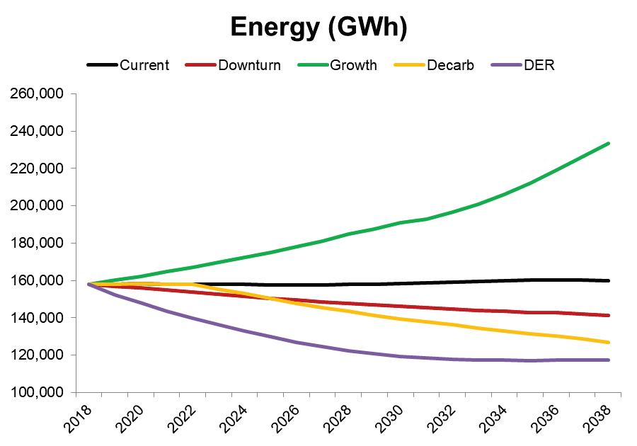
Figure 6-3 shows the forecasted assumptions for natural gas prices. Gas prices are similar for the Current Outlook and No Nuclear Extensions scenarios. The Valley Load Growth and Decarbonization scenarios assume higher gas prices, with the Valley Load Growth increase happening more gradually and the Decarbonization trajectory ratcheting up as assumed regulations take effect The Economic Downturn and
Adoption scenario. The Valley Load Growth scenario projects energy growth of about 2 percent per year.
Each scenario contains unique assumptions around sector forecasts and behind-the-meter impacts that influence load shape, which drives different energy and peak growth patterns. The Current Outlook scenario projects slight peak load growth of about 0.3 percent per year, as does the No Nuclear Extensions scenario. The three scenarios that have declining energy forecasts also have declining peak load forecasts, with the largest peak decline of about -0.7 percent per year in the Rapid DER Adoption scenario. The Valley Load Growth scenario reflects peak load growth of about 1.7 percent per year.
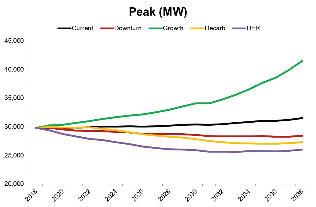
Rapid DER Adoption scenarios assume lower gas prices on somewhat different trajectories.
Figure 6-4 shows the forecasted assumptions for coal prices. Steadily increasing coal prices are forecasted for all scenarios, with modest variations across the scenarios resulting from projected movements in real coal prices and inflation.
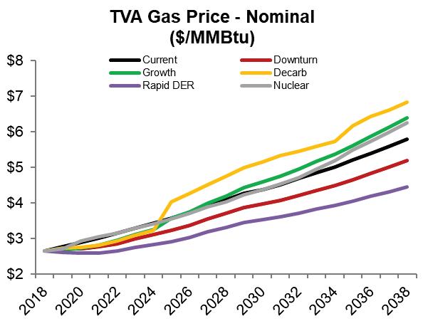
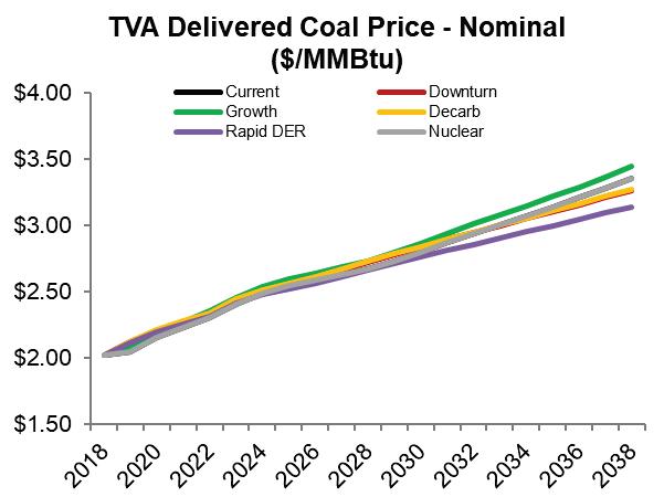
Electricity prices are similar for the Current Outlook and No Nuclear Extensions scenarios. The Valley Load Growth and Decarbonization scenarios assume higher energy prices, with the Valley Load Growth increase happening
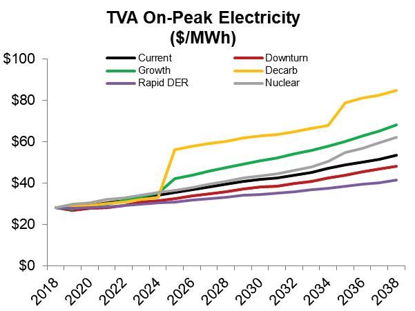
more gradually and the Decarbonization trajectory ratcheting up as assumed regulations take effect. The Economic Downturn and Rapid DER Adoption scenarios assume lower electricity prices on similar trajectories.
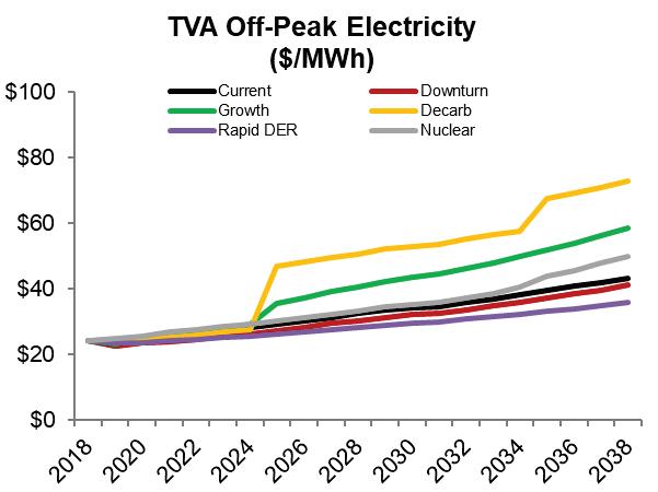
Figure 6-6 shows the forecasted assumptions for CO2 prices. The Current Outlook assumes no carbon penalty, which is also the case in the Economic Downturn, Rapid DER Adoption and No Nuclear Extension scenarios. The Valley Load Growth scenario assumes a modest carbon penalty beginning in 2025 to spur faster adoption of electric vehicles. The Decarbonization scenario assumes a larger carbon penalty driven by regulations or legislative actions that takes effect in 2025 and that is ratcheted up further in 2035.
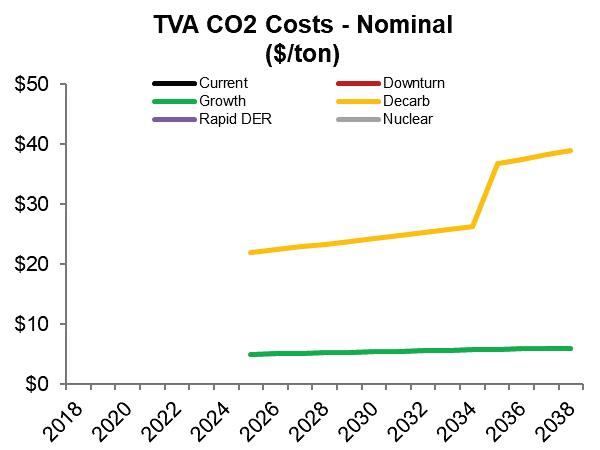
After the scenarios were developed, the next step in the IRP process was to design planning strategies. Scenarios and strategies are very different. Whereas
scenarios describe plausible futures and include uncertainties that TVA cannot control, strategies describe business decisions or approaches that TVA could employ.
Generally speaking, strategies promote certain resources, and in some cases also limit certain resources to support promotion of others. In IRP modeling terms, strategies that constrain how resources are selected may not be fully optimized nor produce plans that have the lowest possible financial cost. When a resource is promoted, the cost of the resource is lowered for model selection within a particular strategy. The full cost (resource and incentive) will be captured in the financial metrics. Several strategies evaluated in this IRP explore the promotion of distributed resources, and the costs of promoting adoption of those resources is shared between TVA and the DER participants These shared costs will be analyzed further using metrics. The process used to develop strategies is described below.
The first step in developing strategies was to identify the key components, or attributes, to be included in each strategy. Ten distinct attributes were identified using input from individuals on the IRP Working Group and comments received during the public scoping period. These attributes are described in Table 6-3
Attributes
Gas Additions
Energy Efficiency
Demand Response
Renewables (Utility Scale)
Storage (Utility Scale)
Distributed Generation/Storage
Description
Limitations on technologies and timing related to the expansion options fueled by natural gas (CT, CC)
Considers energy efficiency programs that are offered by TVA and/or LPCs (excludes impacts from naturally occurring efficiency/conservation)
Considers demand response programs that are offered by TVA and/or LPCs
Limitations on technologies and timing of renewable resources; considers options that would be pursued by TVA or in collaboration with LPCs
Limitations on technologies and timing of storage resources; considers utility scale storage options varying in size or storage capacity
Includes customer-driven resource options or third party projects that are distributed in nature
A ttributes
TVA combined these 10 attributes to initially create seven strategies for consideration by the IRP Working Group After review of the scoping comments, suggestions from members of the IRP Working Group, and further analysis, TVA selected five distinct strategies. Table 6-4 lists the five strategies and their key characteristics.
Strategies
A- Base Case
B- Promote DER
Description and Attributes
• Planning Reserve margins for summer and winter peak seasons are applied, targeting an industry best-practice level of reliability (applies in all strategies)
• No specific resource types are promoted beyond continuation of existing programs as currently forecasted.
• DER is incented to achieve higher end of long-term penetration levels
• New coal is excluded, and all other technologies are available while EE, demand response, distributed generation and storage are promoted
• Programs targeting low-income customers will be part of EE promotion
C- Promote Resiliency
• Small, agile capacity is incented to maximize flexibility and promote ability to respond to short-term disruptions on the power system
• All technologies are available while small modular reactors (SMRs) and small gas additions (aeroderivative turbines, reciprocating engines), demand response, storage and distributed generation are promoted
• Combinations of storage and distributed generation could be installed as microgrids
• Flexible loads and DERs are aggregated to provide synthetic reserves to the grid to promote resiliency
• Targeted electrification and demand and energy management are incented to minimize peaks and troughs and promote an efficient load shape
• All technologies are available but those that minimize load swings, including EE, DR and storage, are promoted
• Programs targeting low-income customers will be a part of EE promotion
• Renewables at all scales are incented to meet growing prospective or existing customer demands for renewable energy
• New coal is excluded, and all other technologies are available while renewables are promoted
Strategy attributes were used in the modeling in several different ways. The Base Case represents least-cost planning with no specific resources promoted and reflects decisions made to date by the TVA Board of Directors. The remaining strategies provide incentives to promote adoption of certain resources, with consideration of market potential, pace of adoption and reserve margin. Resources that were promoted generally received a modeled incentive that improved economics for adoption or selection. In some cases, a resource category may be limited, such as new coal being excluded in the Promote DER and Promote Renewables strategies. Others have temporal restrictions, such as allowing retirements to take effect in a certain year when transmission work to allow plant separation could be completed.
After defining each strategy’s key characteristics, incentive levels were determined to achieve the objectives of the strategy as shown in Figure 6-7 The Strategy Design Matrix provided the roadmap for how resource promotions were applied in capacity planning. Further information on strategy design can be found in Appendix F
The development of resource portfolios was a two-step process. First, an optimized portfolio, or capacity plan, was generated, followed by a detailed financial analysis. This process was repeated for each strategy/scenario combination and for additional sensitivity runs.
Sensitivity runs change one variable in a strategy, such as the level of promotion for a certain resource, to lend insight to the impact of a specific input
TVA uses a capacity optimization model called System Optimizer. 1 This model employs an optimization technique where an “objective function” is minimized subject to a number of constraints.
Energy resources were selected by adding or subtracting assets based on minimizing the present value of revenue requirements (PVRR). PVRR represents the cumulative present value of total revenue requirements for the study period based on an 8 percent discount rate. In other words, PVRR is the present day value of all future costs for the study period, discounted to reflect the time value of money and other factors such as investment risk.
In addition, the following constraints were applied in the optimization runs:
• Balance of supply and demand
• Energy balance
• Reserve margin
• Generation and transmission operating limits
• Fuel purchase and utilization limits
• Environmental stewardship
• Distributed generation/storage adoption.
In order to promote certain resources within a strategy, incentive levels for distributed generation and storage resources were developed to increase adoption in each strategy These resulting adoption levels were modeled as constraints prior to optimizing the balance of the portfolio.
The System Optimizer model uses a simplified dispatch methodology to compute production costs and a “representative hours” approach in which average generation and load values in each representative period within a week are scaled up appropriately to span all hours of the week and days of the months. The least-cost path (based on lowest PVRR) from all feasible states in the study period is identified as the optimized capacity plan.
1 System Optimizer is an industry standard software model developed by ABB
Next, each capacity plan was evaluated using an hourly production costing methodology, which calculated detailed production costs of each plan, including fuel and other variable operating costs. These detailed cost simulations provided total strategy costs and financial metrics that were used in the strategy assessment process.
This analysis was accomplished using a strategic planning software tool called MIDAS 2. MIDAS uses a chronological production costing approach coupled with financial planning data to assess plan cost, system rate impacts and financial risk. It uses a Monte Carlo analysis, 3 which is a sophisticated analytical technique that allows for a better understanding of portfolio performance by testing the variability of key assumptions and expressing portfolio results as a range around an expected case
The total cost for each resource plan (PVRR) was calculated taking into account additional considerations, including the cash flows associated with financing. The model generated multiple combinations of the key assumptions for each year of the study period and computed the costs of each combination. Capital costs for supply-side options were amortized for investment recovery using a real economic carrying cost method that accounted for unequal useful lives of generating assets.
In addition to computation of the total plan cost (PVRR) over the full 20-year study period, a system average cost metric was calculated. This metric provides an alternative view of the revenue requirements for the study period expressed per MWh. It is not intended as a forecast of wholesale or retail rates over the study period. Rather, it was developed to gauge the potential rate impact associated with a given portfolio and provides an indication of relative rate pressure across the strategies being studied. Reviewing this metric in
combination with PVRR and the financial risk measures provides a clearer picture of the cost/risk balance for each resource plan
While scenarios explore step changes in possible futures, stochastic analysis evaluates risk of uncertainty around key planning assumptions for each portfolio. Stochastic analysis of production cost and financials bounds the uncertainty and identifies the risk exposure that is inherent in long-range power supply planning, because the fundamental forecasts used in those studies are inevitably wrong. Variability will result due to supply/demand disruptions, weather, market conditions, technology improvements and economic cycles. A Monte Carlo simulation allows for a better understanding of the richness of possible futures, as well as their likelihoods, so that plans can be made proactively as opposed to reactively. A stochastic model is used to estimate probability distributions of potential outcomes by allowing for simultaneous random-walking variation in many inputs over time.
At TVA, a representative Monte Carlo distribution using Latin hypercube sampling (efficient method for generating probability distributions) comprised of 120 stochastic iterations is developed for each of the scenario/strategy combinations to more fully assess the likely plan costs, generation, and performance for each portfolio To illustrate the iterations, Figure 6-8 shows a trade-off graph comparing PVRR versus CO2 intensity for each iteration of a portfolio as well as the expected value, or average, and the 5th percentile and the 95th percentile, or P(5) and P(95), respectively
A sample stochastic result which compares revenue requirements of two hypothetical portfolios is shown in Figure 6-9. This example illustrates the range of possible results of costs for each portfolio from the P(5) to P(95). The point where the color of the bars changes represents the expected cost for that portfolio.
2 MIDAS is also an ABB product.
3 Monte Carlo analysis is also referred to as stochastic analysis.
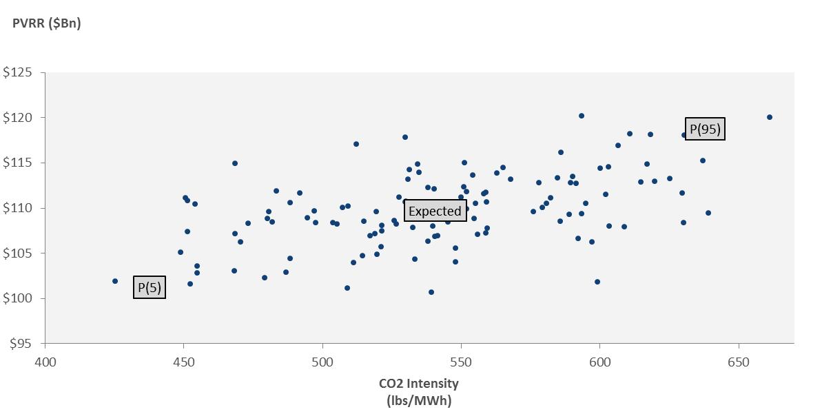
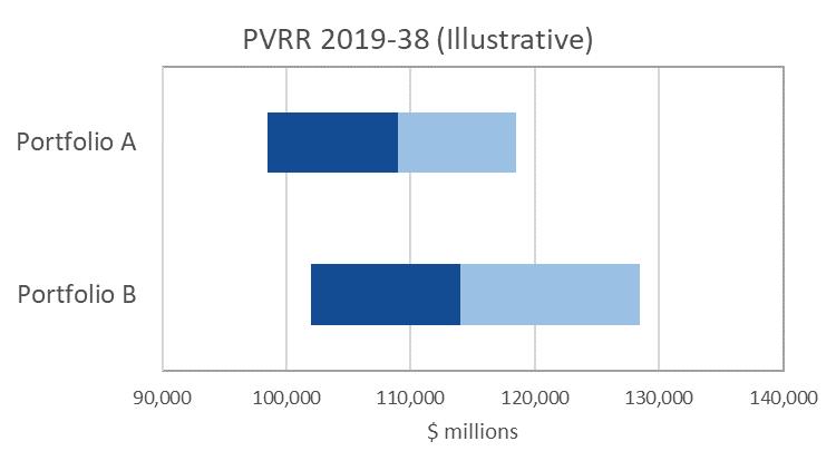
Cost and risk metrics shown later in this report are calculated from the distribution of stochastic iterations
The cost and metrics are primarily the expected values while the risk metrics are functions of the P(5), P(95), and the expected value The MIDAS tool allows TVA to explicitly consider uncertainty and risk exposure in the evaluation of the planning strategies. This analysis is based on applying probability distributions around the
key variables used to frame the scenarios and define assumptions used in the strategies.
The Monte Carlo analysis in MIDAS includes 16 key variables:
• Commodity prices: natural gas, coal, oil, CO2 allowances, electricity price 4
• Financial parameters: interest rates, capital costs, operation and maintenance costs
• Availability: hydro, coal, gas, nuclear, solar, and wind
• Net sales forecast uncertainty: peak and energy, (includes demand, EE, electrification, behind-the-meter solar, and CHP)
The fundamental (expected value) forecasts for these key variables differ across the six scenarios and, as a result, the uncertainty ranges (stochastic envelope) are also different. The evaluation of the uncertainty around the performance of the strategies considers both the variation across the scenarios (different plausible futures) and the probability distribution around the expected forecasts represented by the stochastic envelope. As an example, Figure 6-10 shows these different uncertainty ranges around the TVA peak load forecast.
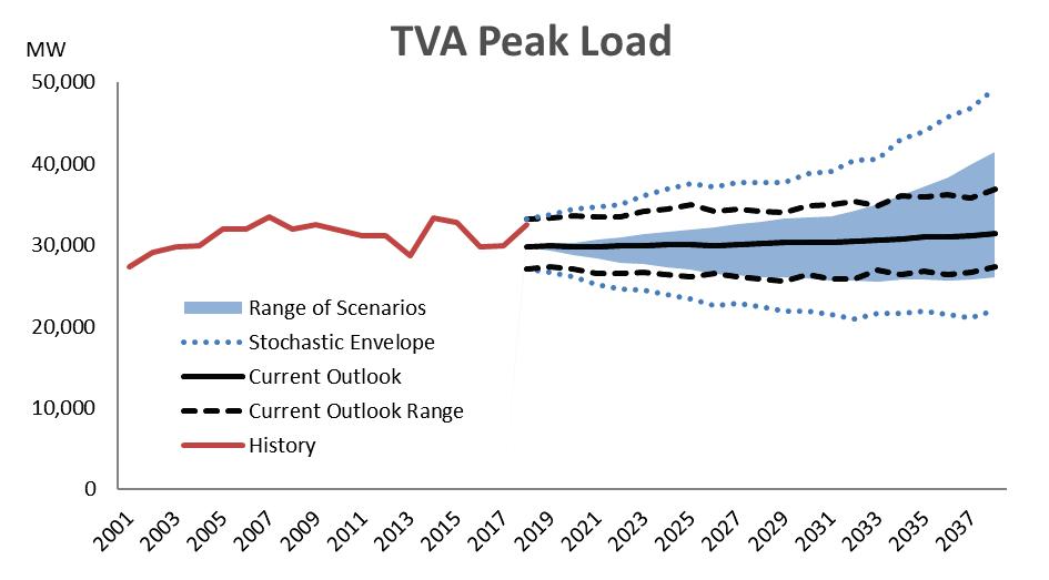
Figure 6-10 shows
(represented by the blue shaded area). For orientation, the Current Outlook scenario’s fundamental forecast and its associated uncertainty range is shown in the black solid and dotted lines. The stochastic envelope, representing the uncertainty ranges from all six scenarios, is shown as the blue dotted line and bounds the uncertainty range evaluated in MIDAS. Each of the 16 key variables has a set of scenario
ranges and stochastic envelopes that ensure a more dynamic assessment of the variability in the performance of each planning strategy.
Modeling multiple strategies within multiple scenarios resulted in a large number of portfolios. So, initially, the portfolio analysis focused on common characteristics
that strategies exhibited over multiple scenarios rather than on specific outcomes in individual portfolios. Strategies that behaved in a similar manner in most scenarios were considered to be “robust” – i.e., more flexible, less risky over the long-term and able to lessen the impacts of uncertainty. Conversely, strategies that behaved differently or poorly in most scenarios were considered more risky with a higher probability for future regret.
The first step in the portfolio evaluation process was to develop a scorecard to assess and compare the performance of strategies in each scenario. The process used to develop an evaluation scorecard is described below.
TVA’s mission and stakeholder concerns related to resource planning were key considerations in developing a set of metrics for use in evaluating the performance of the portfolios generated in the IRP.
To achieve its overall mission of providing low-cost, reliable power to the people of the Valley, TVA focuses on four strategic imperatives, as mentioned previously in Chapter 1. These imperatives are: balancing rates and debt so that TVA maintains low power rates while living within its means; and recognizing the trade-off between optimizing the value of our asset portfolio and being responsible stewards of the Valley’s environment and natural resources
Optimizing TVA’s asset portfolio is the primary purpose of integrated resource planning, but other imperatives also shape the process:
• As part of the financial analysis, a balance sheet and income statement are created for each portfolio to determine the revenue requirements to fund each resource plan.
• A coverage ratio method is used to ensure that the overall debt limit is respected in each optimization run.
• Stewardship obligations are considered in modeling of various compliance requirements, including portfolio optimization which factors in
a carbon penalty and includes key environmental metrics in the assessment of each resource plan (air, water, waste and landuse impacts).
Based on TVA’s strategic imperatives and feedback from stakeholders, five metric categories were selected for use in evaluating the performance of planning strategies:
• Cost , including both the long-range cost of the resource plan as well as a look at average system cost, which is an indicator of possible rate pressure
• Financial Risk , which measures the variation (uncertainty) around the cost of the resource plan by assessing a risk/benefit ratio and computing the likely amount of cost at risk using data from probability modeling
• Environmental Stewardship , which captures multiple measures related to the environmental footprint of the resource plans, including air emissions and water, waste and land use impacts
• Operational Flexibility , which measures how responsive the generation portfolio of each resource plan is by evaluating the portfolio’s ability to ramp up and down to respond to changes in demand
• Valley Economics, which computes the macro-economic effects of the resource plans by measuring the change in real per capita income (where real references the fact that the income streams have been adjusted to remove the impacts of inflation, such that future income streams and present income streams all possess a consistent purchasing capability) and employment compared to a reference case
After establishing the metric categories, the next step was to identify candidate metrics for each category to be used in the scorecard to assess the performance of each strategy in different scenarios
Considering input from the IRP Working Group and Regional Energy Resource Council, TVA selected 14 metrics that clearly and effectively measure the
Category Metric
Definition Cost
PVRR ($Bn)
System Average Cost ($/MWh)
Total Resource Cost ($Bn)
Risk/Benefit Ratio
Risk
Risk Exposure ($Bn)
CO2 (MMTons)
CO2 Intensity (lbs/MWh)
Environmental Stewardship
Water Consumption (MMGallons)
Waste (MMTons)
Land Use (Acres)
Flexible Resource Coverage Ratio
Operational Flexibility
Valley Economics
Flexibility Turn Down Factor
Percent Difference in Real Per Capita Income
Percent Difference in Employment
performance of each portfolio as summarized in Figure 6-11
Total plan cost (capital and operating) expressed as the expected (stochastic) present value of revenue requirements over the 20-year study period
Expected average system cost for the study period, computed as the levelized annual average system cost (annual revenue requirements divided by annual sales)
Total plan cost (capital and operating) expressed as the expected present value of revenue requirements over the study period plus participant cost net of bill savings and tax credits
Area under the plan cost distribution curve between P(95) and expected value divided by the area between expected value and P(5) based on stochastic analysis
The point on the plan cost distribution below which the likely plan costs will fall 95% of the time based on stochastic analysis
Expected annual average tons of CO2 emitted over the study period
Expected CO2 emissions expressed as an emission intensity, computed by dividing emissions by energy generated and purchased
Expected annual average gallons of water consumed over the study period
Expected annual average quantity of coal ash, sludge and slag projected based on energy production in each portfolio
Expected acreage needed for expansion units in each portfolio in 2038
The ratio of flexible capacity available to meet the maximum 3-hour ramp in demand in 2038
Ability of the system to serve low load periods as measured by the percent of must-run and non-dispatchable generation to sales
The change in real per capita personal income expressed as a change from a reference portfolio in each scenario
The change in non-farm employment expressed as a change from a reference portfolio in each scenario
Category Metric Formula
PVRR ($Bn)
Total Resource Cost ($Bn)
System Average Cost ($/MWh)
Risk/Benefit Ratio
Risk Exposure ($Bn)
CO2 (MMTons)
CO2 Intensity (lbs/MWh)
Water Consumption (MMGallons)
Waste (MMTons)
Land Use (Acres)
Flexible Resource Coverage Ratio
Flexibility Turn Down Factor
Percent Difference in Real Per Capita Income
Valley Economics
Percent Difference in Employment
Present Value of Revenue Requirements over Planning Period
PVRR + Participant cost net of savings (bill savings, tax credits)
NPV Rev Reqs (2019−2038)
NPV Sales (2019−2038)
95th PVRR −Expected PVRR
Expected PVRR −5th PVRR
95th Percentile (PVRR)
Average Annual Tons of CO2 Emitted During Planning Period
Pounds CO2 (2019−2038)
MWh Generated & Purchased (2019−2038)
Average Annual Gallons of Water Consumed During Planning Period
Average Annual Tons of Coal Ash and Scrubber Residue During Planning Period
Acreage Needed for Expansion Units in Each Portfolio (2038)
Flexible Capacity Available for Max 3−Hour Ramp in each Strategy (2038)
Capacity Required for Max 3−Hour Ramp in each Scenario (2038)
"Must Run" + "Non−Dispatchable" (2038) Sales (2038)
Percent Difference in Real Per Capita Personal Income Compared to the Base Case (for each scenario)
Percent Difference in Non-Farm Employment Compared to the Base Case
The scorecard metrics selected align with TVA’s mission as shown in Figure 6-13
Once the metrics were selected, the strategy scorecard could be designed. Using a format similar to the 2015 IRP, the scorecard summarizes the performance of an individual planning strategy in each of the scenarios. To evaluate differences within a given scenario, all five scorecards were reviewed. Interpretation of the performance of each strategy is presented in Chapter 7.
Finally, scorecards were populated based on an assessment of overall performance of each strategy in the five metric categories: cost, risk, environmental stewardship, operational flexibility, and Valley economics.
Each metric category was assessed individually and graphics were developed to facilitate interpretation of trends and to identify preliminary observations. Examples of key graphics include a comparison of cost and risk and a comparison of cost and CO2 emissions to enable investigation of possible trade-offs. These observations guided the development of an action plan for further case analysis.
The strategy assessment graphics, along with information about observations from the IRP study and the action plan, can be found in Chapter 8
This chapter describes the findings of the 2019 IRP. The results for 30 distinct portfolios are presented in this chapter, along with the scorecard measures as described in Chapter 6. Throughout the discussion of
results, scenarios are referred to by number and strategies by letter. Portfolios that represent the combination of a scenario and strategy are referred to by the relevant number and letter reference, such as the Current Outlook scenario and the Base Case strategy combination represented as 1A.
The key components of each scenario were translated into a forecast of firm requirements for both summer and winter, based on projected demand and required
reserves in each season. The forecast was used to identify the resulting capacity gap and need for power which drove the selection of resources in the capacity planning model.
Figure 7-1 illustrates the firm requirements forecasts for the six scenarios studied in the IRP.
Firm requirements were greatest in Scenario 3 and lowest in Scenario 5 The remaining scenarios fell within this range. The shape of the firm requirement curves influenced the type and timing of resource additions in the strategies. The timing of resource additions was a
function of the existing system capacity and the impact of the attributes used to define each strategy. Figure 7-2 shows the range of the capacity gaps across the cases.
Capacity expansion plans by strategy are presented below. Further information on the capacity expansion plans is presented in Appendix G – Capacity Plan Summary Charts
Figure 7-3 compares the incremental capacity for all 30 cases by 2038 The ‘incremental’ capacity represents the resources selected to fill the capacity gap referenced above and it includes both resource additions and retirements. The vertical axis is in summer net dependable (SND) megawatts, the capacity that can be applied to firm requirements. While both summer and winter capacity needs and capabilities factored into portfolio optimization, summer
capacity results are being shown throughout the document. Thermal resources have higher net dependable capacities in winter due to ambient temperatures, and hydro generation is typically higher in winter than in summer Additionally, solar resources have higher capacities in summer, while wind resources have higher capacities in winter. The results for each strategy are grouped together, and incremental capacity additions are grouped by resource type (i.e., nuclear, hydro, coal, solar, etc.).
Scenarios 4 and 5 had the lowest demand forecasts and therefore the least amount of incremental capacity. Conversely, Scenario 3 had the highest demand and therefore resulted in the most incremental capacity.


Highlights of capacity additions by 2038 for all 30 cases are summarized below by resource type:
Nuclear: No new nuclear was selected in any portfolio other than in 6C, where two SMRs totaling 1,200 MW were added as part of Strategy C to replace one of three Browns Ferry units. All three Browns Ferry units were retired in all strategies in Scenario 6
Hydro: No new hydro was selected in any portfolio, driven primarily by the competitiveness of forecasted solar prices.
Coal : No new coal plants were selected. In carbonconstrained and lower load futures, additional coal generation was retired beyond that currently planned, up to about 2,200 MW (including the impact of accelerated retirements) depending on the scenario and strategy combination. Strategy D resulted in the most additional coal retirements.
Natural Gas : Natural gas additions varied more significantly than other resources and depended on the forecasted load in each scenario and the strategic focus. Scenario 3 cases had the highest addition of
Gas CT capacity, up to 8,400 MW, while no additional Gas CT capacity was chosen in the Scenario 5 cases In scenarios with lower load expectations, such as Scenario 2, 4, and 5, some older existing CT capacity was retired Gas CC capacity additions were similar in Scenario 1 and the declining load scenarios (2, 4 and 5) at 1,500 MW. Scenario 6 cases have 2,500 MW in incremental Gas CC capacity, while Scenario 3 cases have the highest Gas CC expansion ranging from 7,400 to 9,800 MW
Renewables: Figure 7-3 shows the non-hydro renewable assets in summer net dependable megawatts, which is the amount of firm capacity that can be expected at the system peak. No new wind was selected. Solar expansion is significant in all cases, ranging from 2,600 to 6,000 MW on a summer net dependable capacity basis, or about 4,000 to 9,000 MW of nameplate capacity Portfolios include varying amounts of utility (single-axis tracking) and distributed solar, as certain strategies (B, C and E) promote distributed solar. Solar expansion is highest, on average, in Strategy E
Storage: Storage additions range from 0 to 5, 300 MW depending on strategic focus. Most storage additions are utility-scale batteries, with mechanical selected in some instances. Additions are highest in Strategy D, moderately high in Strategies C and E, and relatively small in Strategy B. Without promotion, no storage is added in Strategy A.
EE: The amount of energy efficiency added is consistent within a strategy and ranges from about 20 MW in several strategies to a high of 85 MW in Strategy D. Load forecasts include projections for more efficient electricity usage driven by codes and standards and changes in consumer behavior, with variation across the scenarios as applicable.
DR : The incremental demand response averages about 75 MW across all 30 cases, reaching a high of 300 MW in some cases. These DR additions complement


current interruptible pricing products and programs assumed to continue in all cases.
The capacity plans (firm supply plus incremental capacity) are presented below. Further information on the capacity plans is presented in Appendix G –
Figure 7-4 compares the capacity plans in 2038 for all 30 cases. The capacity plans represent the total resource portfolios available to meet firm requirements, shown in summer net dependable (SND) megawatts, grouped by strategy, and segmented by resource type.
Since Scenarios 4 and 5 have the lowest demand forecasts, these scenarios typically have the lowest capacity. Conversely, Scenario 3 has the highest demand, resulting in the highest capacity.


Highlights of capacity plans in 2038 are summarized below by resource type:
Nuclear: Nuclear capacity is the same in all cases, with the exception of Scenario 6 where Browns Ferry Nuclear units are retired. In that scenario, the Strategy
C portfolio has 1,200 MW higher nuclear capacity than the other portfolios due to the addition of two SMRs in that strategy.
Hydro: Hydro capacity is the same across all portfolios.
Coal : Coal capacity is the same or less than currently planned, as no coal was added. Strategy D results in the lowest coal capacity on average across the scenarios. Scenario 4 results in low coal capacity across all strategies.
Gas : Gas capacity is lower in the declining load scenarios (2, 4 and 5) and is significantly higher in the Scenario 3 cases. Strategy D has the lowest gas additions, driven by the promotion of storage.
Renewables: Solar becomes a significant part of all 30 capacity portfolios, and is highest on average in Strategy E. Portfolios include varying amounts of utility and distributed solar, as certain strategies (B, C and E) promote distributed solar. No additional wind is selected in any portfolio.
Storage: Storage capacity includes the existing Raccoon Mountain Pumped Storage plant, and strategies that promote storage add to this existing storage amount. Strategy D has the highest storage capacity, and Strategies C and E also see increases.
EE: EE capacity is similar across portfolios and highest in Strategy D cases. Load forecasts include projections for more efficient electricity usage driven by codes and standards and changes in consumer behavior, with variation across the scenarios as applicable.
DR : DR capacity includes current interruptible pricing products and programs assumed to continue in all cases, with additions averaging 75 MW and up to 300 MW in some cases
Energy plans resulting from the associated capacity plans are presented below. Further information on the energy plans is presented in Appendix G – Capacity Plan
Figure 7-5 compares the energy plans in 2038 for all 30 cases. The energy plans represent the energy expected from the economic dispatch of the resources available in each capacity plan, shown in terawatt-hours (TWh), grouped by strategy, and segmented by resource type.
Energy patterns across strategies and scenarios generally vary for similar reasons as noted in the discussion of capacity plans. Nuclear generation is the same in most portfolios, except for Scenario 6 cases, and h ydro generation is the same in all portfolios. Coal generation reflects no additional coal but some retirements, and is the lowest on average in Strategies C and D and in Scenario 4 cases Gas generation is similar on average across strategies, and is appreciably higher in Scenario 3 cases. Solar generation is a larger part of the portfolio in all cases, and is highest in Strategy E Strategy D results in the highest generation (discharge) from storage, followed by Strategies C and E. Finally, energy contribution of EEDR is modest overall and highest in Strategy E


As described in Chapter 5, both utility and distributed scale options for solar and storage resources are offered in the 2019 IRP. The approach used to model accelerated adoption of distributed resources using an incentive mechanism is discussed further in Appendix C. Figure 7-6 shows incremental solar and storage
capacity by 2038, delineating additions as utility or distributed scale. Strategy D results in the highest combined levels of solar and storage at all scales due to a high promotion of storage, followed by Strategies C and E As the Decarbonization and Rapid DER Adoption scenarios already include a high penetration of distributed solar and storage, there is no ability to incent further adoption through a TVA strategy.


Another way to look at solar additions is by the nameplate capacity, or designed maximum output under ideal conditions. Figure 7-7 shows the nameplate
solar additions across the strategies and scenarios. Solar additions are highest on average in Strategy E, followed closely by Strategies C and D. Strategies A and B have a similar level of solar additions on average
The vast majority of thermal additions across portfolios were natural gas. Several new natural gas options were offered in the 2019 IRP, including aeroderivatives (smaller, highly flexible CTs) and a distributed gas option (combined heat and power, or CHP). The approach used to model accelerated adoption of CHP


is discussed further in Appendix C. Figure 7-8 shows incremental gas capacity by 2038, delineating additions as CC, Frame CT, Aero CT, or CHP. Strategy D has the lowest gas additions overall, while Strategy C swaps Frame CTs for Aero CTs due to the promotion of small, agile resources in that case. In Scenario 6, two 600 MW SMR units are promoted in Strategy C to replace one Browns Ferry nuclear unit


Given the focus on exploring distributed resources in this IRP, another interesting view is a summary of distributed energy resource additions resulting from incentives through a TVA strategy, beyond what occurs behind the meter in any scenario. Figure 7-9 shows
incremental DER capacity by 2038, with delineations for distributed solar, distributed storage, CHP, and EEDR. Incremental DER capacity is highest in Strategy B, as might be expected, but is also higher in some of the Strategy C and E cases.


Programmatic options for energy efficiency (EE), demand response (DR), and beneficial electrification (BE) are offered as resource options in all strategies and are promoted to the greatest extent in Strategy D.
Figures 7-10 and 7-11 summarize the incremental EEDR and BE capacity in Strategy D at several points in time throughout the 20-year study period. Even in strategies where programmatic DER has little or no incentive, similar patterns play out over time but at generally lower levels.
Regarding EE, programs related to reducing energy consumption for residential, commercial and industrial entities are selected early in the study period. As the impacts of codes and standards materialize in the load forecast and consumer behaviors evolve, there is less need for TVA programmatic EE. The competitiveness of solar prices also played a role in driving less need for EE There is the potential to expand EE programs for low-income residential consumers, who have less opportunity to adopt energy efficient technologies. These programs are expanded throughout the Valley
and incented highly in Strategy D. Cumulative capacity from this program increases through time, leveling out toward the end of the study period.
Relative to DR, programs related to reducing energy consumption at the TVA system peak are also selected early in the study period. DR resources include programs that aggregate and control residential space conditioning and water heating around the peak. In the latter half of the study period, impacts begin to roll off and other resources are selected to meet peaking needs, especially storage that is highly incented in this case.
For BE, a similar pattern is exhibited as for EEDR, excluding the low-income program. Programs that target electrification which help optimize the load shape by filling valleys and shaving peaks are selected early in the study period. Commercial & Industrial options are most attractive given their relatively lower cost. Levels of BE selected are comparatively higher in general than EE and vary more across scenarios. The highest levels of BE occur in Scenario 5, where differences in peaks and valleys in the load shape are the most extreme


Strategy A: Base Case is TVA’s least-cost optimization plan that applies no additional incentives or targets. Resources are chosen economically to meet the reserve margin constraint for reliability
Figure 7-12 presents the modeled capacity results for Strategy A. The capacity portfolios show the summer net dependable megawatts in 2038. The nuclear portfolio is the same in all scenarios, except for Scenario 6 where Browns Ferry units are retired. Hydro capacity is the same in all cases. Coal capacity is the same in all scenarios, except for Scenario 4, where carbon regulation leads to additional coal retirements Solar assets are added beginning in the mid-2020 time frame, and continue to be added throughout most of
the planning horizon Including hydro, renewables account for 18 percent of the capacity portfolio on average. Natural gas assets increase over time, beginning with Gas CC additions that could be achieved through renewal of existing contracts, acquisitions or builds. These are augmented by Gas CT additions in Scenario 3 and 6 cases With current cost projections and no promotion in Strategy A, no storage appears in any portfolios Energy efficiency increases modestly in all scenarios, with impacts lessened as efficiencies from codes and standards increase. Demand response increases similarly across scenarios, with some differentiation due to load shape and strategic focus.
Figure 7-13 shows the energy portfolios that correspond to the capacity charts in Figure 7-12.
Nuclear energy remains the same over time across the cases, with the exception of the Scenario 6 case where energy from the retired Browns Ferry units is replaced primarily with solar and gas generation. Hydro energy remains the same across portfolios. Coal generation decreases over the planning horizon as units are retired and declines further in lower load cases, especially in Scenario 4 Solar generation increases substantially in all cases, with the highest increases seen in Scenario 3 and 4 portfolios. Including hydro, renewables account for 20 percent of total generation on average. Natural gas generation varies with load and strategic focus,
Scenario 1: Current Outlook
Scenario 2: Economic Downturn
Scenario 3: Valley Load Growth
Scenario 4: Decarbonization
Scenario 5: Rapid DER Adoption
Scenario 6: No
with the highest gas generation seen in the Scenario 3 and 6 cases. Demand response, which produces low energy volumes, has been combined with the energy efficiency into one group termed EEDR Incremental EEDR contributes a small amount to the portfolio, with increasing impacts from codes and standards reflected in the load forecast without additional TVA incentives. Strategy A results in 61 percent carbon-free generation in 2038 on average
Scenario 2: Economic Downturn
Scenario 3: Valley Load Growth
Scenario 4: Decarbonization
Scenario 5: Rapid DER Adoption
Scenario 6: No Nuclear Extensions
Scenario 1: Current Outlook TWh
Nuclear Hydro Coal Gas Renewables Storage EEDR
Strategy B: Promote DER focuses on increasing the pace of DER adoption by incenting distributed solar and storage, combined heat and power, energy efficiency and demand response. Promotions are first applied, and then the balance of the system is optimized in a least-cost manner. The approach used to model increased adoption through an incentive mechanism is discussed further in Appendix C.
Figure 7-14 shows the capacity resources added by 2038 in Strategy B across the six scenarios. The results from this strategy are very similar to Strategy A with a few notable differences. Distributed solar is promoted in this strategy and generally replaces a portion of lower
cost utility solar. Distributed storage is also promoted, replacing a portion of demand response but at a higher cost. Finally, CHP is promoted, driving slightly lower utility-scale gas additions
Figure 7-15 shows how the energy portfolios for Strategy B play out driven by the capacity changes and other factors in the scenarios Including hydro, renewables account for 20 percent of total generation on average. Strategy B results in 61 percent carbonfree generation in 2038 on average, similar to Strategy A.
Scenario 1: Current Outlook
Scenario 2: Economic Downturn
Scenario 3: Valley Load Growth
Scenario 4: Decarbonization
Scenario 5: Rapid DER Adoption
Scenario 6: No Nuclear Extensions
Scenario 1: Current Outlook
Scenario 2: Economic Downturn
Scenario 3: Valley Load Growth
Scenario 4: Decarbonization
Scenario 5: Rapid DER Adoption
Scenario 6: No Nuclear Extensions
Strategy C: Promote Resiliency incents higher adoption of small, agile capacity to increase the operational flexibility of TVA’s power system, while also improving the ability to respond locally to short-term disruptions Promotions are first applied, and then the balance of the system is optimized in a least-cost manner. The approach used to model increased adoption through an incentive mechanism is discussed further in Appendix C.
Figure 7-16 presents the
2038 for Strategy C. The hydro portfolio is the same as in Strategy A. Nuclear capacity is the same as in Strategy A, with the exception of Scenario 6 where 1,200 MW of SMRs are added to replace one Browns Ferry nuclear unit. C oal capacity is the same across all scenarios, except for Scenario 4 in which carbon regulation leads to additional coal retirements. When more coal is retired, solar capacity increases at both utility and distributed scales. Storage additions are promoted, resulting in somewhat lower gas capacity
Scenario 1: Current Outlook
Scenario 2: Economic Downturn
Scenario 3: Valley Load Growth
Scenario 4: Decarbonization
Scenario 5: Rapid DER Adoption
Scenario 6: No Nuclear Extensions
Scenario 1: Current Outlook
Scenario 2: Economic Downturn
Scenario 3: Valley Load Growth
Scenario 4: Decarbonization
Scenario 5: Rapid DER Adoption
Scenario 6: No Nuclear Extensions
additions on average. EEDR volumes remain similar across the scenarios in this strategy.
Figure 7-17 shows the resulting energy portfolios for Strategy C driven by the capacity changes and other factors in the scenarios Including hydro, renewables account for 22 percent of total generation on average. Strategy C results in 63 percent carbon-free generation in 2038 on average, compared to 61 percent in Strategy A.
Strategy D: Promote Efficient Load Shape incents targeted electrification, demand response, and energy management to optimize load shape, including programs targeting low-income energy efficiency. Promotions are first applied, and then the balance of the system is optimized in a least-cost manner.
Figure 7-18 shows the capacity resources added by 2038 in Strategy D across the six scenarios. The nuclear and hydro portfolios are the same as in Strategy A This strategy results in the highest amount of coal retirements on average. That capacity is replaced with a combination of solar, storage and gas additions, with a high penetration of solar achieved in all cases. Storage is promoted to the greatest degree
Scenario 1: Current Outlook
Scenario 2: Economic Downturn
Scenario 3: Valley Load Growth
Scenario 4: Decarbonization
Scenario 5: Rapid DER Adoption
Scenario 6: No Nuclear Extensions
in this strategy, resulting in the highest storage capacity overall. The storage additions drive the lowest need for gas capacity, especially CT peaking units. The highest EE volumes are seen in this strategy, and DR volumes are similar to Strategy A by 2038, as the promotion of storage meets peaking needs.
Figure 7-19 shows the corresponding energy portfolios for Strategy D driven by the capacity changes and other factors in the scenarios. Including hydro, renewables account for 22 percent of total generation on average. Strategy D results in 61 percent carbonfree generation, similar to Strategy A
Scenario 1: Current Outlook
Scenario 2: Economic Downturn
Scenario 3: Valley Load Growth
Scenario 4: Decarbonization
Scenario 5: Rapid DER Adoption
Scenario 6: No Nuclear Extensions
Strategy E: Promote Renewables incents renewables at all scales to meet growing prospective or existing customer demands for renewable energy Promotions are first applied, and then the balance of the system is optimized in a least-cost manner. The approach used to model increased adoption through an incentive mechanism is discussed further in Appendix C.
Figure 7-20 presents the total capacity portfolios in 2038 for Strategy E. The nuclear and hydro portfolios are the same as in Strategy A. Coal capacity is the same across all scenarios, except for Scenario 4 in which carbon regulation leads to additional coal retirements. The highest levels of solar additions are seen in this strategy across all scenarios, averaging nearly 6,000 MW summer NDC and 9,000 MW
nameplate. Including hydro, renewables account for 20 percent of the capacity portfolio on average. Storage is also promoted, resulting in a comparable level of storage additions as in Strategy C, and similarly reducing the need for gas capacity additions. EEDR volumes remain similar across the scenarios in this strategy, also resembling Strategy C.
Figure 7-21 shows the corresponding energy portfolios for Strategy E driven by the capacity changes and other factors in the scenarios. Including hydro, renewables account for 22 percent of total generation on average. Strategy E results in 62 percent carbon-free generation in 2038 on average, compared to 61 percent in Strategy A
Scenario 1: Current Outlook
Scenario 2: Economic Downturn
Scenario 3: Valley Load Growth
Scenario 4: Decarbonization
Scenario 5: Rapid DER Adoption
Scenario 6: No Nuclear Extensions
Scenario 1: Current Outlook
Scenario 2: Economic Downturn
Scenario 3: Valley Load Growth
Scenario 4: Decarbonization
Scenario 5: Rapid DER Adoption
Scenario 6: No Nuclear Extensions
The fully populated scorecards for each of the five strategies are included in this section (see Chapter 6 for a discussion about the development of the scorecard template). Each strategy scorecard contains the metric values for that particular strategy in each of the six scenarios modeled in the IRP. The metric values are based on the combination of the portfolio optimization and uncertainty analysis work applied to each of the strategies under consideration.
The scorecard for Strategy A (Base Case) is shown in Figure 7-22. The highest PVRR is the Valley Load Growth due to the large build-out to meet firm requirements. The highest system average cost is the Rapid DER Adoption. The Valley Load Growth has the highest risk exposure driven by higher loads, and has the highest CO2 emissions, water consumption, solid waste production, and land use Strategy A has the best flexibility performance across all scenarios. Because the Valley Economics metric uses Strategy A as the reference case in computing impacts, the change in per capita income is 0 percent for this strategy.
The scorecard for Strategy B (Promote DER) is shown in Figure 7-23 These results are very similar to those shown for Strategy A across the metrics with the
exception of total resource cost. Higher total resource cost is driven by the promotion of distributed resources that tend to have less economies of scale.
The scorecard results for Strategy C (Promote Resiliency) are shown in Figure 7-24. PVRR and system average costs are slightly higher than Strategy A and B due in part to promotion of storage Strategy C has moderate financial risk compared to other strategies. This strategy has the lowest environmental impact
overall, due to the largest amount of coal retirements across scenarios, but high land use due to the large amount of solar expansion. Flexibility scores are comparable to the results for Strategies D and E.
The Strategy D (Promote Efficient Load Shape) scorecard is shown in Figure 7-25 This strategy has the highest PVRR and system average cost due to the highest promotion of storage and is mid-range among the strategies in total resource cost. Strategy D has the highest risk exposure across the strategies. It has low
environmental impact overall, but higher land use due to a large solar expansion. Flexibility scores are comparable to the results for Strategies C and E.
metric values are shown in Figure 7-26 PVRR and system average costs are slightly higher than Strategy A and B. Similar to Strategy C, Strategy E has moderate financial risk
compared to other strategies. It has low environmental impact overall, but higher land use due to a large solar expansion. Flexibility scores are comparable to the results for Strategies C and D.
Figure 7-27 shows a comparison of how each strategy scored across all scenarios by metric
Based on the results of the modeling, TVA made the following observations about incremental capacity across the portfolios
• There is a need for new capacity in all scenarios, even in low load futures, to replace expiring or retiring capacity
• Solar expansion plays a substantial role in all futures, driven by its attractive energy value beginning in the mid-2020 time frame
• Gas, storage and demand response additions provide reliability and/or flexibility across all seasons
• No baseload resources (designed to operate around the clock) are added, except for the promotion of SMRs in one case
• Additional coal retirements occur in certain futures, especially in a carbon-constrained world
• EEDR levels are relatively similar across the portfolios, with EE opportunity decreasing as efficiency impacts from codes and standards increase over time
• In all cases, TVA will continue to provide for economic growth in the Tennessee Valley.
These observations are further explored in the assessments presented in Chapter 8.
This chapter explains the strategy assessments and summarizes the results. Areas where additional study may be needed and next steps in the IRP process are also discussed. Throughout the assessment discussion, scenarios will be referred to by number and strategies by letter. Portfolios that represent the combination of a scenario and strategy will be referred to by the relevant number and letter reference, such as the Current Outlook scenario and the Base Case strategy combination represented as 1A.
To assess the performance of the five planning strategies (explained in Chapter 6 and highlighted here), TVA used scorecard data to conduct four assessments:
• Cost and risk
• Environmental stewardship
• Operational flexibility
• Valley economics
Strategy A: Base Case
Strategy B: Promote DER
Strategy C: Promote Resiliency
Strategy D: Promote Efficient Load Shape
Strategy E: Promote Renewables
The cost and risk assessment was aimed at gaining a better understanding of the relative performance of different strategies in terms of total plan costs and financial risk.
The cost assessment was based on three scorecard metrics:
• PVRR ($Bn) – Total plan cost (capital and operating) expressed as the expected (stochastic) present value of revenue requirements over the 20-year study period
• System Average Cost ($/MWh) – Expected average system cost for the study period, computed as the levelized annual average system cost (annual revenue requirements divided by annual sales)
• Total Resource Cost ($Bn) – Total plan cost (capital and operating) expressed as the expected present value of revenue requirements over the study period plus participant costs net of bill savings and tax credits
These metrics allow a comparison of the cost and financial risks associated with different planning strategies. (See Chapter 6, section 6.2.2, for more information on metrics, including the formulas used to compute them.)
Figure 8-1 provides a comparison of portfolio results for PVRR and Total Resource Cost (TRC), which also includes net participant costs
PVRR for the 20-year study period is similar across the strategies, with Strategies A and B typically lower and Strategy D typically the most expensive. Average system costs are also similar, with similar trends as PVRR across the strategies. Total Resource Cost has more variation, with Strategy A the least expensive and Strategy B typically the most expensive.
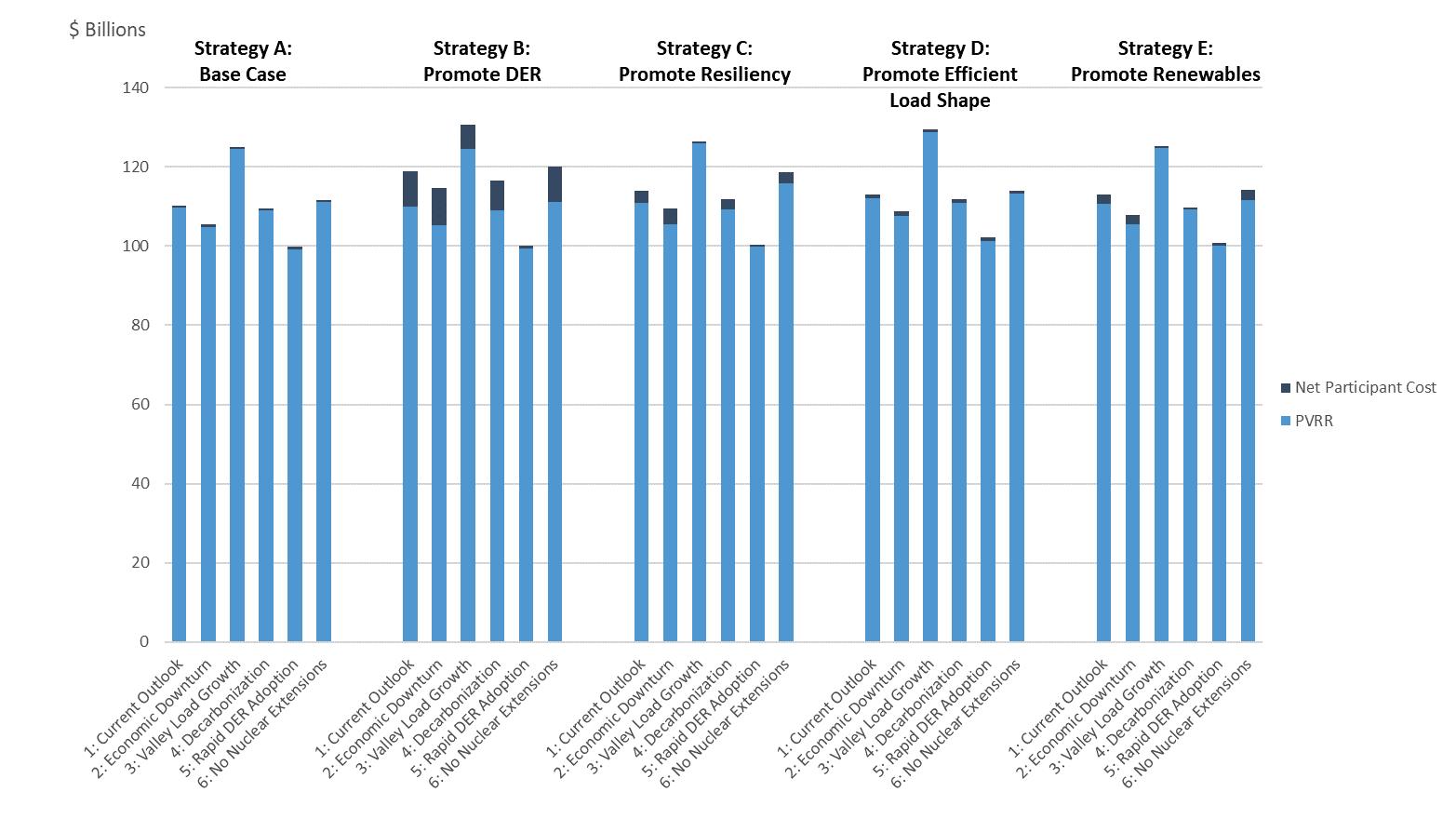
Another view of PVRR and TRC that is helpful to consider is the range of outcomes around the expected case for each strategy, as shown for Scenario 1 (Current Outlook) in Figures 8-2 and 8-3. The lower end of each bar is the best case (lowest cost) outcome from the uncertainty analysis; the upper end is the worst
case (highest cost) outcome; and the expected value is the point of transition between the two colored sections of each bar
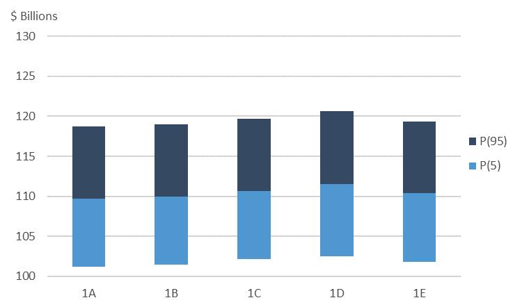
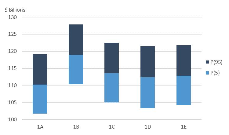
Figure 8-4 shows the results for the system average cost metric for Scenario 1 (Current Outlook) The blue bar represents the system average cost values for the 20-year study period (2019-2038), the orange bar represents the values for the first 10 years (2019-2028), and the gray bar represents the values for the second 10 years (2029-2038).
Over the 20-year study period, system average cost follows the PVRR relationships with Strategies A and B the lowest cost, Strategies C and E mid-range, and Strategy D the highest cost.
During the first 10-year period, the system average cost is very similar across all five strategies. In the second 10-year period, there is more variation. Strategies A and B are the lowest, followed by Strategy E, then Strategy C, and finally Strategy D, which exhibits the
highest system average cost due to the highest promotion of storage. Within and across metric categories, evaluating tradeoffs can be insightful.
Figure 8-5 shows the tradeoff between PVRR and system average cost across the portfolios. For example, the Valley Load Growth scenario (Scenario 3) has the largest expansion and largest capital cost requirement (highest PVRR), but also has the greatest amount of energy sales. This higher amount of sales reduces system average cost. Conversely, the Rapid DER Adoption scenario (Scenario 5) has the lowest expansion but also has the lowest amount of sales, resulting in the highest system average cost (i.e., spreading cost over a fewer number of sales).
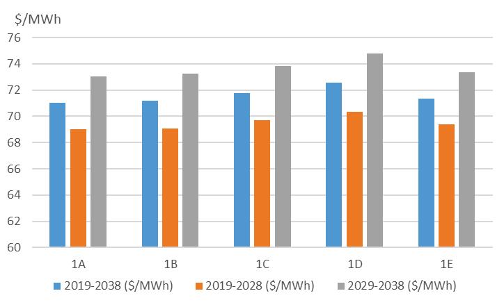
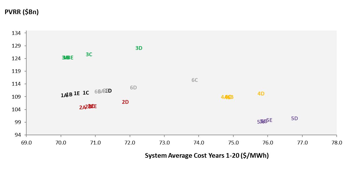
While scenarios explore step changes in possible futures, stochastic analysis evaluates risk of uncertainty around key planning assumptions for each portfolio, as described in Chapter 6. Stochastic analysis of production cost and financials bounds the uncertainty and identifies the risk exposure inherent in long-range
resource planning driven by supply/demand disruptions, weather, market conditions, technology improvements and economic cycles.
Two additional metrics, leveraging the use of stochastic analysis, were used to assess the risk of each strategy:
• Risk / Benefit Ratio – Area under the plan cost distribution curve between P(95) and expected value divided by the area between expected value and P(5) based on stochastic analysis
• Risk Exposure – The point on the plan cost distribution below which the likely plan costs will fall 95 percent of the time based on stochastic analysis
Figure 8-6 shows a comparison of the risk/benefit ratios and risk exposures for the Current Outlook. For these metrics, lower values indicate better performance
where the benefits outweigh the risks and overall risk exposure is less. Risk/benefit scores less than 1.0 indicate that costs are more likely to be less than the expected value, and scores higher than 1.0 indicate costs are more likely to be greater than expected value. Risk exposure represents the worst case outcome and is useful in determining which strategies present higher financial risks overall
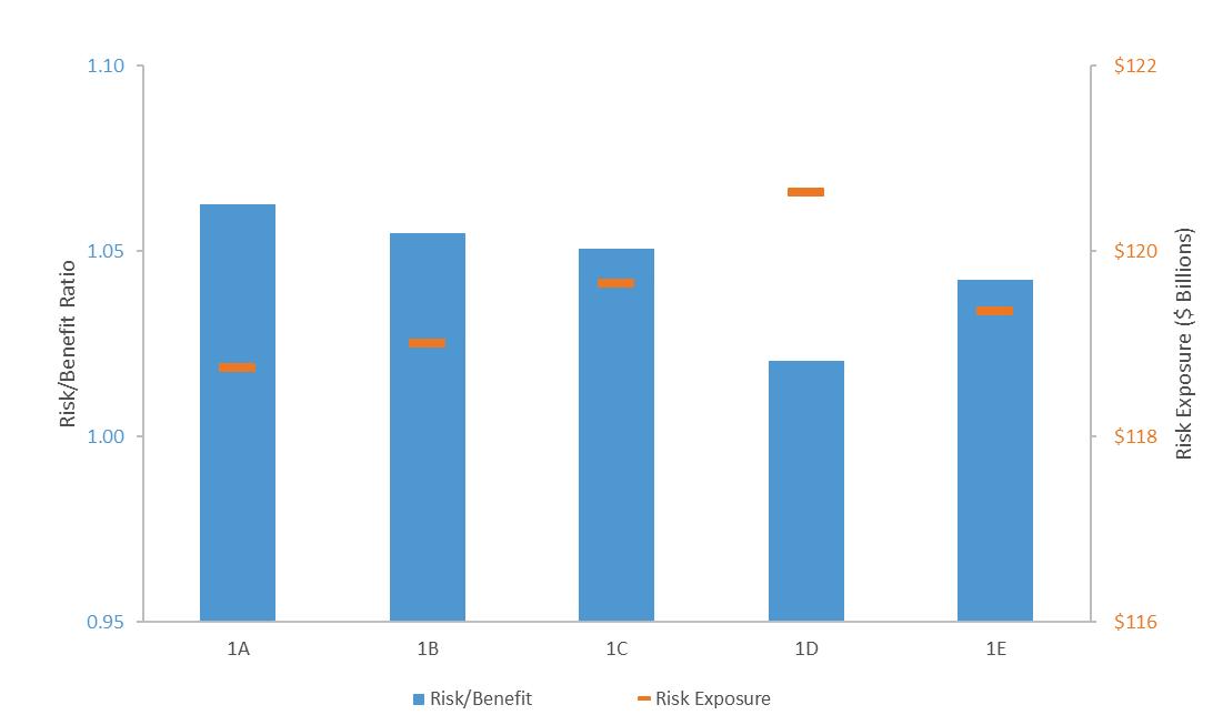
Strategies with lower costs generally have lower risk exposure. Strategy A has the lower risk exposure but least favorable risk/benefit ratio, while Strategy D has the opposite profile Other strategies have moderate risk overall. Most portfolios have risk/benefit ratios between 1.0 and 1.1, indicating that risks typically outweighed the benefits. Some portfolios in declining load cases have risk/benefit scores less than 1.0, indicating less financial risk in lower load scenarios.
Relative to risk exposure, Strategies A and B have the lowest levels while Strategies C and E have mid-range risk exposure. Strategy D carries the highest financial
exposure and is the most risky, about $2 billion more at stake on average than in Strategy A. Overall, these results indicate that strategies which constrain resource selection have higher risk exposure. Strategies which promote a resource that is significantly higher in cost relative to alternatives, such as storage, will have higher cost and risk exposure.
Another way to assess cost and financial risk is to combine the cost and risk scores so that an analysis of tradeoffs can be performed. Figure 8-7 shows cost/risk trade-offs based on comparisons of risk exposure to TRC
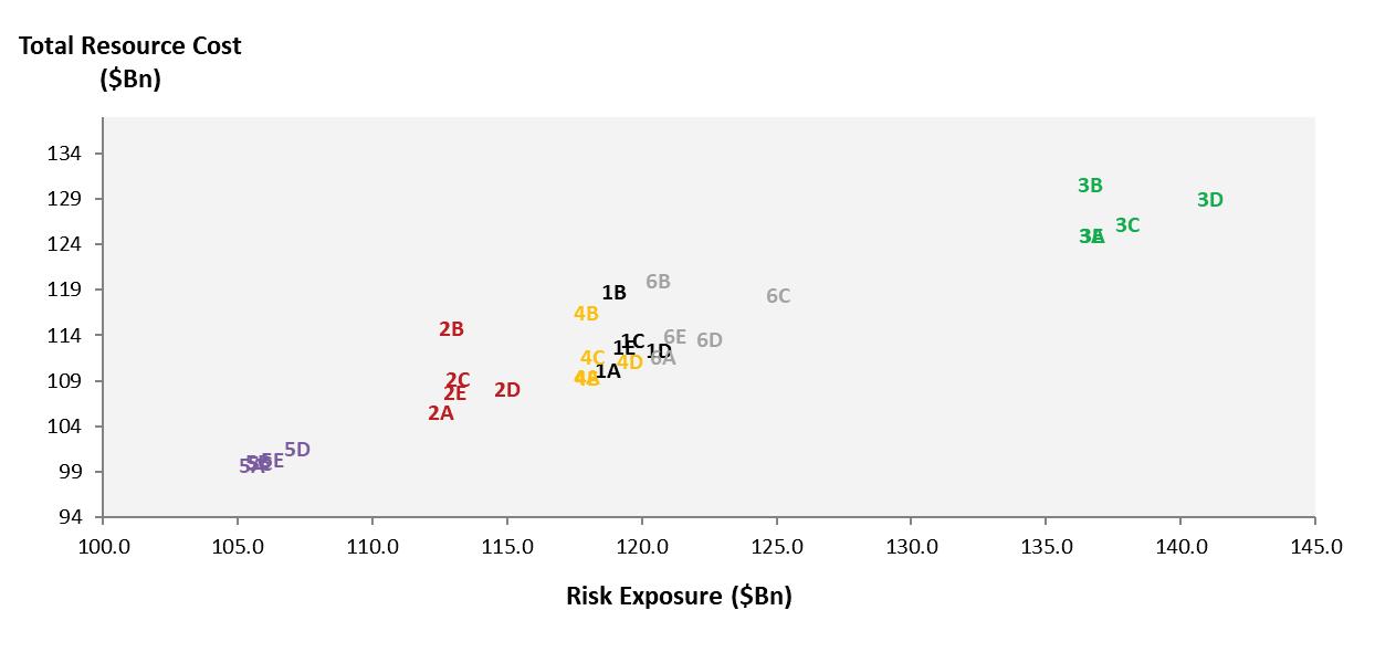
These charts reinforce the cost and risk assessment results Generally, within a scenario, Strategy A has lower cost and risk exposure, Strategy B has the highest cost (on a TRC basis) with mid-range risk exposure, and Strategy D has mid-range cost and highest risk exposure The exception is the 6C case, which forces in two SMRs to partially replace the loss of the Browns Ferry units.
More information on financial metrics and the range around expected cases (stochastics) for all portfolios can be found in Appendix H.
As described in Chapter 6, strategy scorecards include five measures for environmental stewardship performance:
• CO2 Tons – the expected annual average tons of CO2 emitted over the study period
• CO2 Intensity – the expected CO2 emissions expressed as an emission intensity, computed by dividing emissions by energy generated and purchased
• Water consumption – the expected annual average gallons of water consumed over the study period
• Waste – the expected annual average quantity of coal ash, sludge and slag based on energy production in each portfolio
• Land Use – the expected acreage needed for expansion units in each portfolio in 2038
Figure 8-8 shows the average environmental impact for Scenario 1 (Current Outlook) across all strategies. More information about the development of these metrics can be found in Appendix I
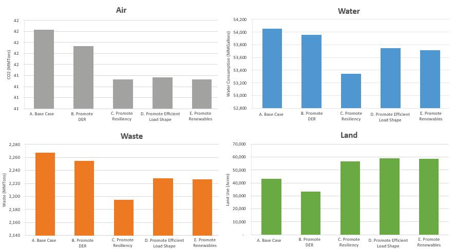
All strategies show improvement in air, water and waste compared to the current resource portfolio, with Strategy C the most favorable. All strategies show increased land use compared to the current resource portfolio driven by various levels of solar expansion. Strategies that promote solar tend to have favorable environmental profiles, except for increased land use. While overall land use is higher for solar facilities on a per MW basis, the impacts to the land are generally low level and have the potential to be readily returned to the previous condition or use.
Strategy C has the lowest environmental impact with respect to air, water and waste. Strategy A has the highest environmental impact overall but low land use. The other strategies generally fall somewhere in
between, except for land use where Strategy B has the lowest acreage.
Another helpful view is a comparison of CO2 intensity across all 30 portfolios. As shown in Figure 8-9, the scenario has the greatest influence on CO2 intensity, with variations across strategies as described in the Current Outlook example. Range of stochastic results are included in Appendix I
Figure 8-10 shows trade-offs between system average cost and CO2 intensity across all portfolios. The scenario that materializes will drive CO2 intensity at relatively similar system average cost, regardless of the strategy.
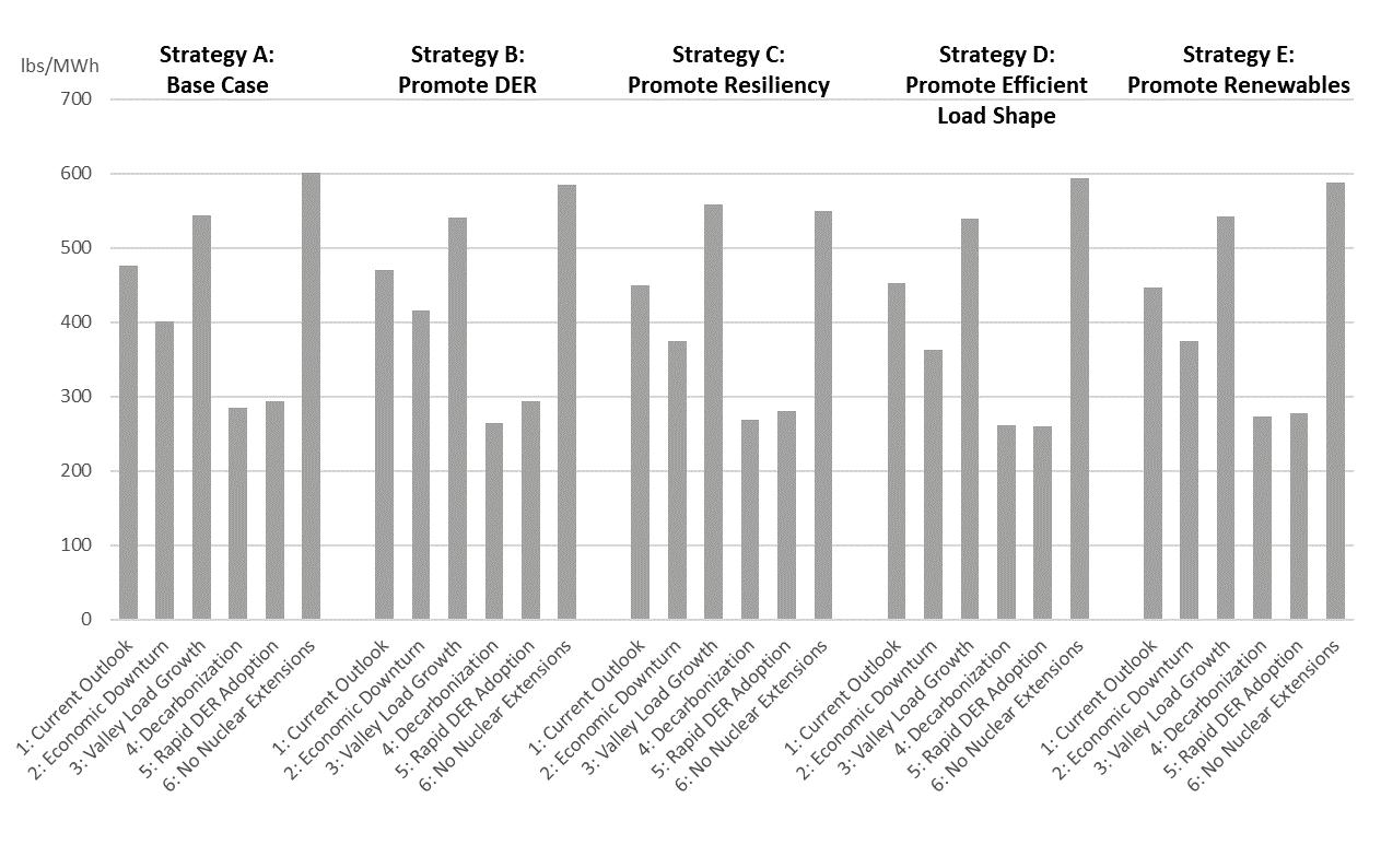
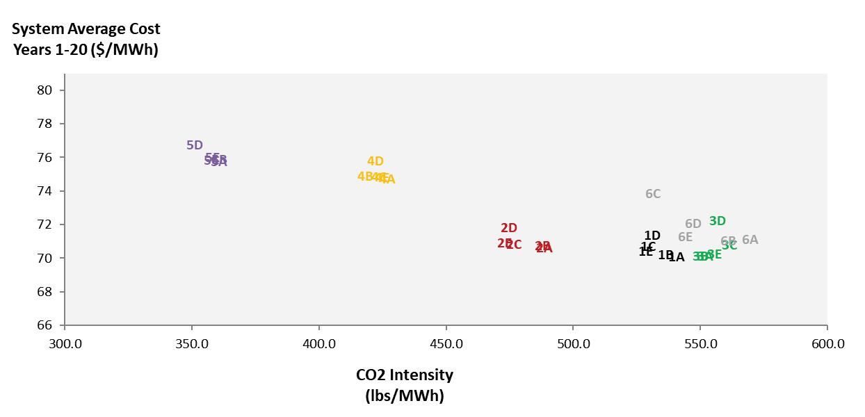
As described in Chapter 6, understanding system flexibility is a focus in this IRP. Strategy scorecards include two measures of operational flexibility:
• Flexible Resource Coverage Ratio – the ratio of flexible capacity available to meet the maximum 3-hour ramp in demand in 2038
• Flexibility Turn Down Factor – the ability of the system to serve low load periods as measured by the percent of must-run and nondispatchable generation to sales.
TVA views system flexibility – the ability to cover rapid changes in load demand and to serve low load periods – as a key future consideration for long-range resource
planning. This is especially true as the resource mix shifts from conventional, fully dispatchable central station units toward more diverse and dispersed generating assets that introduce more intermittency.
This is the first time TVA has used flexible resource coverage as a metric to assess the performance of a resource portfolio. TVA based this measure in part on research of other utilities and independent system operators in an effort to represent a portfolio’s ability to meet rapid changes in demand.
Figure 8-11 shows a comparison of flexible resource coverage ratio and flexibility turn down factor for the Current Outlook. Figure 8-12 displays cost and flexibility trade-offs across all portfolios
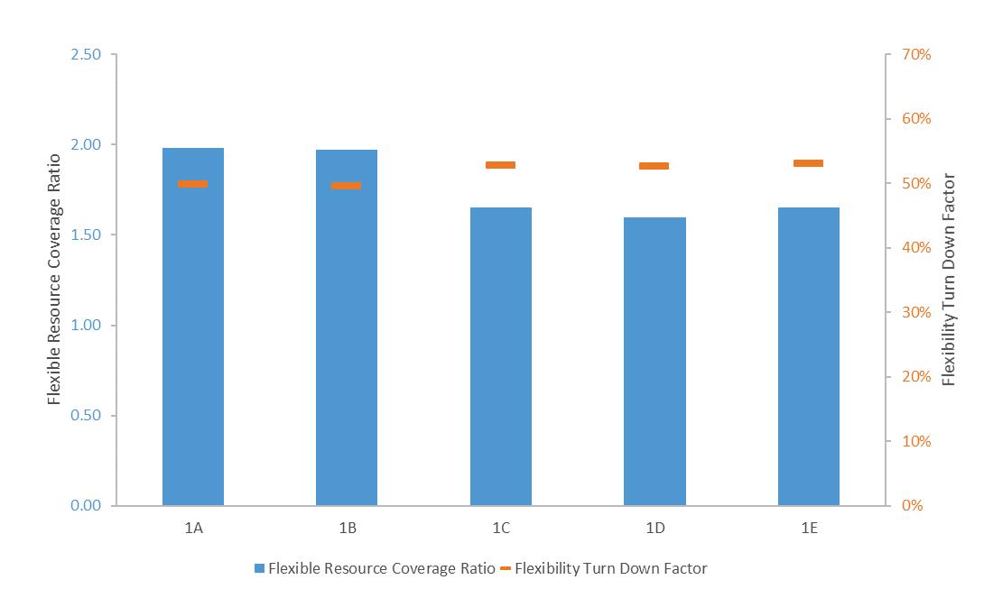
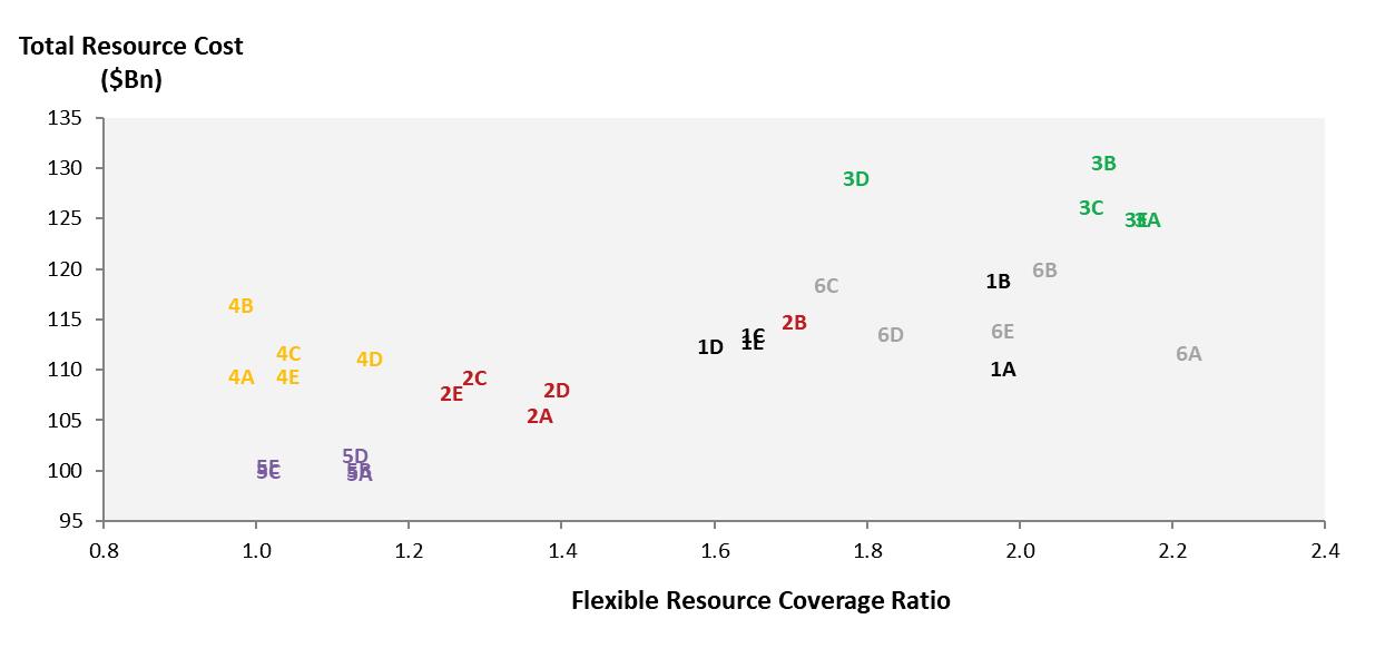
TVA’s analysis indicates that Strategies A and B result in a more flexible system than other strategies on average. Strategies that drive more solar expansion tend to have lower flexibility. In portfolios where nuclear units are retired (Scenario 6) and replaced in part with gas units, overall system flexibility increases. In general, portfolios with a higher percentage of non-dispatchable resources will have relatively less ability to respond to unexpected load swings.
The impact of different planning strategies on the Valley economy was assessed based on two measures:
• Percent Difference in Real Per Capita Income –the change in real per capita personal income expressed as a change from a reference portfolio in each scenario
• Percent Change in Non-Farm Employment –the change in employment expressed as a change from a reference portfolio in each scenario
The reference portfolio is the level of impact to per capita income or employment in Strategy A in each scenario. More details about how TVA has computed this macro-economic impact can be found in Appendix
J. All strategies have comparable impacts on the Valley economy based on these two standard measures.
Strategy D consistently outperformed the reference income level across all scenarios. This is likely due to the retention of more investment in the Valley under this strategy driven by the commitment to energy efficiency, which results in increased investment in the Valley relative to other resource options. However, the overall variation in per capita income estimates is very small across the strategies, in part due to changes in other factors such as underlying population growth (e.g., in some cases employment increases are matched or even exceeded by larger corresponding increases in Valley population), changes in the composition of employment (increased total non-farm employment yet declining manufacturing employment), and/or changes in regional inflation levels due to higher electricity costs. Furthermore, the scale of TVA incremental investments across the various scenarios and strategies are modest in relation to the overall size of the Valley economy. This suggests that the Valley Economics metric is unlikely to be a key definitive determinate when selecting a preferred target power supply mix.
Based on analysis of scorecard results, TVA makes the following observations about metric performance across the portfolios:
• The strategy that most leverages utility-scale resources is the most economic and has the lowest risk exposure (Strategy A)
• The strategy that most leverages distributed resources has the highest Total Resource Cost (Strategy B).
• The strategy that most leverages storage has the highest PVRR, driven by current projections for storage prices (Strategy D).
Metric Category Assessment Observations
Cost
Risk
Environmental Stewardship
Operational Flexibility
Valley Economics
• Strategies that most leverage solar and coal retirements have lower environmental impact overall, but higher land use (Strategies C, D and E)
• Strategies that drive more solar expansion tend to have lower operational flexibility (Strategies C, D and E)
• All strategies have comparable impacts on the Valley economy as measured by real per capita income and employment.
The overall performance of the five planning strategies is explained in more detail below, by metric category in Table 8-1 and by strategy in Table 8-2.
• PVRR is similar across the strategies, with Strategy D typically the most expensive
• Average system costs are also similar, with Strategies A and B typically lower and Strategy D typically the highest
• Total Resource Cost has more variation, with Strategy A the least expensive and Strategy B typically the most expensive
• Strategies with lower costs generally have lower risk exposure
• Strategy A has the lowest risk exposure but least favorable risk/benefit ratio, while Strategy D has the opposite profile
• Other strategies have moderate risk overall
• All strategies show improvement in air, water and waste categories compared to the current resource portfolio, with Strategy C the most favorable
• All strategies show increased land use compared to the current resource portfolio driven by various levels of solar expansion, with the exception of Strategy B
• Strategies A and B result in a more flexible system than other strategies, on average
• Strategies that drive more solar expansion tend to have lower flexibility
• In portfolios where nuclear units are retired (Scenario 6) and replaced in part with gas units, overall system flexibility increases
• All strategies have comparable impacts on the Valley economy as measured by real per capita income and employment
Strategy Assessment Observations
Strategy A:
Base Case
Strategy B: Promote DER
Strategy C: Promote Resiliency
Strategy D: Promote Efficient Load Shape
• Lowest PVRR, Total Resource Cost, and System Average Cost across scenarios
• Lowest risk exposure, but highest risk/benefit ratio
• Highest environmental impact overall, but low land use
• Best flexibility performance across scenarios
• Similar to Strategy A in PVRR and System Average Cost, but most expensive with respect to Total Resource Cost
• Risk exposure similar to Strategy A, with moderate risk/benefit profile
• Higher environmental impact overall, but lowest land use
• Flexibility performance comparable to Strategy A
• Mid-range in PVRR, System Average Cost, and Total Resource Cost
• Moderate financial risk
• Lowest environmental impact overall, but higher land use
• Moderate flexibility, comparable to Strategies D and E
• Highest PVRR and System Average Cost due to promotion of storage, and mid-range in Total Resource Cost
• Highest risk exposure across the strategies
• Low environmental impact overall, but higher land use
• Moderate flexibility, comparable to Strategies C and E
Strategy E: Promote Renewables
• Mid-range in PVRR and System Average Cost, but lower in Total Resource Cost (second only to Strategy A)
• Moderate financial risk
• Low environmental impact overall, but higher land use
• Moderate flexibility, comparable to Strategies C and D
Each IRP case represents a combination of expectations about the future environment TVA operates in and potential strategies TVA could employ that result in unique resource portfolios. When analyzing results from the draft IRP, TVA identified issues that warranted further evaluation prior to finalizing the study. In addition, TVA received helpful stakeholder input from the IRP Working Group and the Regional Energy Resource Council (RERC), as well as through comments received from the public during the comment period.
Many of the questions raised by TVA and stakeholder review focused on certain key assumptions that could influence results. To explore the impacts of changes in key assumptions and to inform the recommendation ranges in Chapter 9, TVA evaluated sensitivities related to the following categories:
• Natural gas prices
• Storage, wind, CHP, and SMR capital costs
• Greater EE and DR market depth
• Integration cost and flexibility benefit
• Pace and magnitude of solar additions
• Higher operating costs for coal plants
• More stringent carbon constraints
• Variation in climate
Sensitivity analyses are typically run as variations from the Base Case strategy in the Current Outlook scenario, except where noted, to isolate the impact of a change in one key assumption.
Natural gas generation makes up a significant part of TVA’s existing fleet, and several types of gas generation
are offered as expansion options. Changes in natural gas prices change the variable cost of gas units and may change the economics of different types of gas capacity relative to other resource options. Two standard deviations above and below the expected value were simulated in the Current Outlook. Figure 813 shows the range of natural gas prices for the IRP scenarios and for two standard deviations above and below the Current Outlook forecast.
Higher natural gas prices increase the cost of gas generation, making the generation of competing resources more valuable. Solar is projected to become economic compared to gas beginning in the mid2020s, resulting in 5,900 MW nameplate of solar expansion in the base plan. In the high gas sensitivity, about 2,050 MW nameplate of additional solar capacity is added by 2038 compared to the base case, bringing total nameplate solar expansion to about 8,000 MW in this case. Other changes in the expansion plan include the addition of 55 MW of new hydro, as well as reduced electrification programs driven by the overall higher operating cost for the fleet. The Total Resource Cost increased by about $6 billion due to higher fuel costs. Carbon emissions increased 21 percent driven by an overall increase in coal capacity factors.
Lower natural gas prices improve the economics of gas generation, especially higher efficiency CCs In the low gas sensitivity, no solar is added, which represents a reduction of 5,900 MW in nameplate solar compared to the base case. Additionally, about 2,000 MW of CT capacity is replaced by CC capacity to better leverage lower gas prices. This sensitivity does not take into account customer demand for renewables that would likely drive more solar additions than economics would dictate. The Total Resource Cost decreased by about $6 billion due to lower fuel costs. Carbon emissions decreased 21 percent driven by an overall increase in gas capacity factors.
Several resource options that were promoted in an IRP strategy were not selected based on economics in any of the primary portfolios. Of particular interest were battery storage, wind, CHP, and SMRs. TVA, stakeholder groups, and the public expressed interest in understanding how much lower the costs of these resources would need to be for the resource to become economic. TVA performed a breakeven analysis to determine how the IRP costs for battery storage, wind, CHP, and SMR compared to the benefits those units could provide to the system.
The IRP cost is the levelized cost of the resource using Current Outlook assumptions. To determine the benefits the resource could provide to the system, TVA added the resource to the portfolio in the earliest year available at zero cost and calculated the levelized benefit in $/MWh This approach effectively describes the value of these resources in terms of the avoided energy and capacity from competing resources. As IRP cost approaches breakeven cost, the resource is more likely to be selected in a portfolio.
Even though the IRP assumed a downward trajectory in costs, utility-scale battery storage was not selected based on economics. Due to the varying ways that augmentation and warranty costs can be included in the initial capital investment or paid on an ongoing basis as a fixed cost, direct comparisons between benchmarks requires calibration. As described in Appendix C, TVA matched storage additions to solar additions in strategies where storage was promoted to explore the potential impacts of storage on overall portfolio results. Additionally, TVA performed a breakeven analysis. As battery storage is a higher-value resource, the breakeven value to the system is higher than for wind or CHP. However, using current projections for utility scale battery storage costs, IRP costs are still triple the breakeven value. TVA will
continue to monitor rapidly evolving battery storage technologies for improving economics.
Although a small amount of CHP did appear in the Promote DER strategy portfolios, the IRP stakeholder working group expressed interest in understanding the breakeven value for CHP without promotion. Analysis indicates that IRP costs for CHP are double the breakeven value. CHP systems also provide steam for space heating, driving additional value for the end-use customer that was not included in the breakeven analysis.
Wind from both outside and inside the Valley has challenging economics. Out-of-Valley wind must be imported to TVA across interconnected systems, driving significant transmission expense. In-Valley wind has lower intensity and efficiency, driving lower capacity factors and higher effective costs. Additionally, the production tax credit is set to expire which will increase costs for all wind options, and IRP costs assume no decreasing technology curve. TVA performed a breakeven analysis for out-of-Valley wind, which had the better cost profile. Analysis indicates that IRP costs for wind are triple the breakeven value.
A further sensitivity case was evaluated to test the effects of a substantially lower wind forecast than the IRP cost assumptions. While IRP assumptions for wind costs were in the range of the National Renewable Energy Laboratory (NREL) ATB mid-case forecast, TVA used the lower bound of NREL’s mid-case adjusted to nominal dollars for this sensitivity Lower prices could be the result of technology improvements, cost efficiencies, tax incentives, or a reduction in transmission costs. Figure 8-14 compares the IRP wind cost assumptions and the NREL lower mid-case cost trajectory, and it includes solar cost projections as an additional reference point.
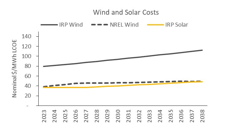
In the NREL lower mid-case sensitivity, 4,200 MW nameplate of wind capacity was added by 2038. Because wind resources contribute about a third of their nameplate capacity toward meeting winter reserve margin targets, some gas additions were displaced early in the plan. If the lower wind cost materializes, wind would also compete with solar in the latter part of the plan and displace about 3,100 MW nameplate of solar by 2038, reducing solar additions roughly by half.
SMR investment would be capital-intensive and represent first-of-a-kind technology deployment at utility scale. Given this, TVA performed a breakeven analysis to help understand the cost gap and inform ongoing discussions with the Department of Energy, a stakeholder that may be willing to share in costs and risks associated with potential SMR deployment. SMRs were evaluated assuming operation beginning in 2028 and running through the end of the study window in 2038. A limitation of this analysis is that capitalintensive resources have long economic lives, and two thirds of SMR economic life would be outside the study window. Analysis indicates that IRP costs for SMRs are more than double the breakeven value. Refinements in design may improve SMR costs, but cost and risk sharing are essential to close the gap.
Across the primary IRP cases, the amount of available programmatic EE and DR is limited in yearly additions and total cumulative volumes based on projected opportunity. TVA performed a sensitivity to determine the potential impact if EE and DR market depth was greater than projected. Additional tiers of programmatic EE and DR were offered at incrementally increasing costs and with no cumulative volume limit. Analysis indicates about 2,100 MW of additional EE and DR was economic compared to the base case, if higher volumes could be realized at assumed costs. Additional EE and DR displaces about 2,200 MW nameplate of solar and about 2,000 MW of CT capacity. An assumed increase in EE and DR market depth results in a similar PVRR, higher system average cost, and 10 percent lower carbon emissions.
Integration cost is the sub-hourly economic signal used to represent the cost of balancing an intermittent resource with dispatchable resources. This cost is not recognized in hourly planning models Conversely, flexibility benefit is the sub-hourly value that highly flexible and dispatchable resources have that also isn’t recognized in hourly models. More detail can be found
on integration cost and flexibility benefit in Appendix D. Reflecting a sub-hourly integration cost and flexibility benefit was a recent addition to our modeling framework, so TVA performed a sensitivity to evaluate the impact of removing them from our models. Removing integration cost and flexibility benefit drove a very similar end result for resource selection, indicating that these costs and benefits alone do not drive macrolevel decision making but would inform evaluation of specific deals, contracts, and decisions.
Limits on the pace, timing, and magnitude of resource additions are common in modeling, as they serve to create more realistic resource plans. For example, the ability to construct or contract resources may be limited by the market or by the ability of operations to integrate new resources into the portfolio. Annual limits in a model that has perfect foresight also prevents overoptimizing resource selections in any single year. TVA, stakeholder groups and the public raised questions about the impact of limitations on solar, in particular. Solar was limited in three ways in the primary cases, as follows:
• 2023 earliest online date, driven by August 2019 IRP publication date and subsequent time required for interconnection requests and environmental permitting
• Annual addition limit of 500 MW nameplate, reflecting other utilities’ experience with average annual solar additions
• Cumulative limit of 10,000 MW nameplate based on the study window time frame and system turndown capability
TVA performed a sensitivity to evaluate the impact of accelerating solar additions to as early as 2021 to align with two programs to support accelerated renewable investment launched after the IRP base case was established. These programs include the Renewable Investment Agreement (RIA) and the Flexibility Research Project (FRP) pilot. RIA supports utility scale buildouts for large commercial and industrial customers, and FRP supports community solar in
partnership with LPCs. In this sensitivity, TVA reflected recent solar signings of about 700 MW scheduled to come online in 2020/2021 (contracted after the IRP base case was established) and assumed 500 MW per year of accelerated solar additions thereafter until economic solar additions pick up in the mid-2020s. Analysis of potential acceleration indicates about 1,100 MW nameplate of additional solar by 2038 compared to the base case.
TVA also performed a sensitivity that doubled the annual addition limit to 1,000 MW and removed the cumulative limit. This analysis indicates a similar result of about 1,100 MW nameplate of additional solar by 2038 compared to the base case.
In discussions about the solar sensitivities evaluated in the Current Outlook, stakeholder groups inquired if results might be different in other scenarios. TVA performed an additional sensitivity to test the impact of increasing annual and cumulative limits in the Valley Load Growth base case (3A). Higher electricity demand with no additional base load resources added would lower the turndown pressure in the growth case. This additional sensitivity was run with an annual addition limit of 1,000 MW and a cumulative limit of 14,000 MW, which is roughly the difference between the growth scenario load profile and the output of baseload nuclear and hydro resources adjusted for pumped storage ability to shift some baseload. Analysis indicates 6,000 MW nameplate of additional solar compared to the growth scenario base case, or 14,000 MW nameplate of solar additions in total. Other expansion changes include 1,000 MW of CCs replaced with CTs.
When reviewing results of the primary cases, TVA and stakeholders had questions about the ongoing operating costs for TVA’s coal fleet Aging coal units expected to operate more frequently outside their design, driven by low gas prices and increasing renewables on the system, have a greater risk of substantially increased operating costs. To assess the potential impact, TVA performed a sensitivity simulating a high trajectory for operations and maintenance costs
and capital costs for the coal plants, as well as higher environmental spend. Unit performance assumptions remained the same as in the base case, while total non-fuel costs were increased by over 60 percent on average on a present value basis.
Analysis indicates the potential for about 2,200 MW of coal to be retired by 2028. As the retired coal capacity had relatively low capacity factors overall, CTs were the preferred replacement resource.
When reviewing results of the primary cases, stakeholders inquired about the potential impact of a higher than projected carbon penalty in the Decarbonization scenario.
To assess this, TVA performed a sensitivity off the Decarbonization base case (4A) that doubled the carbon penalty to $40-80/ton and reflected the cascading impact in natural gas and power price forecasts. Figures 8-15 through 8-17 shows a comparison of the key assumptions in the Current Outlook and Decarbonization base cases compared to the double decarbonization sensitivity case.
Analysis indicates an acceleration of about 2,200 MW of coal retirements that were already present in the Decarbonization base case. CC expansion was accelerated, displacing coal generation, and 175 MW of hydro generation was added by 2038.
Stakeholders also expressed interest in understanding how variation in climate may impact capacity expansion plans. Based on an USEPA report (USEPA 430-F-16004, "What Climate Change Means for Tennessee"), the effects of climate change may mean hotter, drier summers and warmer, wetter winters. Hotter and drier summers will reduce the output of thermal and hydro resources and increase loads. On the other hand, a warmer and wetter winter will decrease loads and increase hydro generation. TVA performed a sensitivity to gauge the impact of a 3° F increase in the average annual temperature across the Tennessee Valley, coupled with changes in seasonal rainfall.
Analysis for this sensitivity indicates that the TVA system would become summer peaking. CT additions are accelerated to replace the impact of derated coal and nuclear capacity in the summer until about 2,100
MW nameplate of additional solar can be added to help maintain summer reserve margins. Total Resource Cost increased by about $3 billion due to the increased summer peak and thermal derates in the summer, while carbon emissions improved slightly due to increased solar and hydro generation and decreased coal generation.
The sensitivity cases TVA performed that have the potential to impact capacity expansion are summarized below in Figure 8-18. Capacity expansion impacts are shown by resource type, with increases highlighted in green and decreases highlighted in red. The results from the sensitivity cases were considered in developing the IRP Recommendation
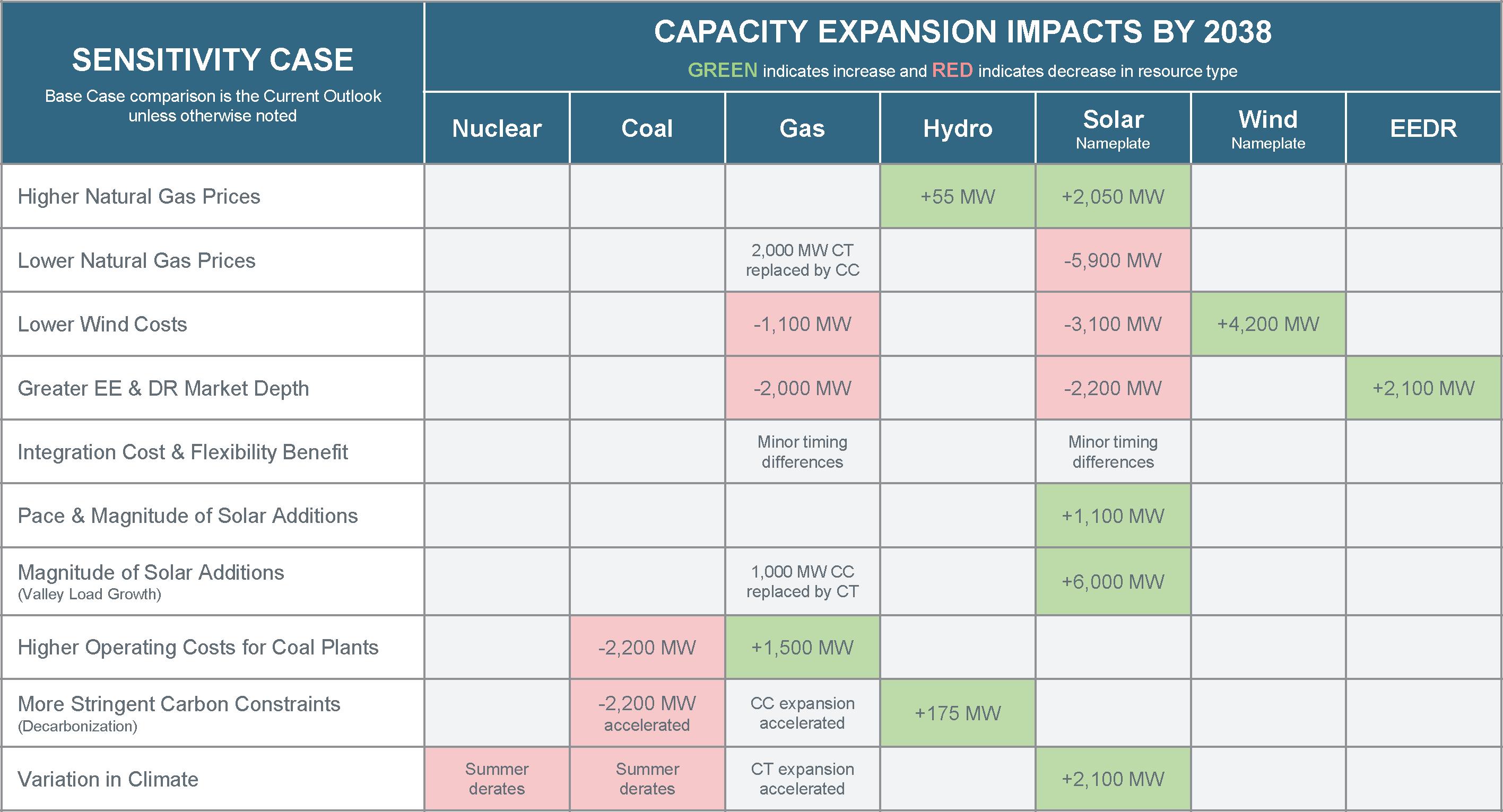
The Tennessee Valley Authority’s 2019 Integrated Resource Plan (IRP) will guide TVA in making decisions about the energy resources used to meet future demand for electricity. Having a long-range resource plan enables us to provide low-cost, reliable and clean electricity to the people we serve. The plan is a crucial element for success in a constantly changing business and regulatory environment that will better equip us to meet many of the challenges facing the electric utility industry in the coming years.
TVA used an integrated, least-cost framework considering multiple views of the future to determine how potential resource portfolios could perform in different market and external conditions. TVA’s goal is to identify an energy resource plan that performs well under a variety of future conditions, taking into account cost, risk, environmental stewardship, operational flexibility and Valley economics.
TVA conducted the IRP process in a transparent, inclusive manner that provided numerous opportunities for public education and participation. The analyses performed in this IRP study relied on industry-standard models and incorporated best practices while using an innovative methodology to more fully evaluate the role of distributed energy resources in the power supply mix. Resource cost and performance input data were independently validated.
The IRP study demonstrates that TVA power will continue to be low-cost, reliable and clean into the future. Our resource additions will build on TVA’s existing diverse asset portfolio.
Study results show:
• There is a need for new capacity in all scenarios to replace expiring or retiring capacity
• Solar expansion plays a substantial role in all futures
• Gas, storage and demand response additions provide reliability and/or flexibility
• No baseload resources (designed to operate around the clock) are added, highlighting the need for operational flexibility in the resource portfolio
• Additional coal retirements occur in certain futures (such as lower load, higher operating cost, and carbon-constrained worlds)
• Energy Efficiency (EE) levels depend on market depth and cost-competitiveness
• Wind could play a role if it becomes costcompetitive (including transmission)
• In all cases, TVA will continue to provide for economic growth in the Tennessee Valley.
TVA assessed the performance of the five planning strategies using metrics to evaluate cost and risk, environmental stewardship, operational flexibility and effects on Valley economics. TVA’s observations about strategy performance include the following:
• The scenario TVA finds itself operating in has more impact on overall results than the strategy or strategies TVA implements.
• All strategies evaluated have positive aspects but also have unique tradeoffs to consider.
The IRP results, including the 30 primary cases and the sensitivity cases, provide a robust set of potential resource additions and retirements evaluated in the IRP from which the final recommendation was derived. The Recommendation takes into account customer priorities around power cost and reliability across different futures, along with environmental stewardship and Valley economics. Implementing the least-cost resource plan with these priorities in mind will help ensure TVA continues to fulfill its mission to serve the people of the Tennessee Valley.
In developing a recommendation from the study, TVA has elected to establish guideline ranges for key resource types (owned or contracted) that make up the
target power supply mix. This general planning direction is expressed over the 20-year study period while also including more specific direction over the first 10-year period. In order to distill the considerable number of cases evaluated through the original scenario and strategy analysis, and the sensitivity cases, the recommendation uses ranges that are centered on results obtained under the Current Outlook scenario. The other scenario and sensitivity results provide a sense of how the recommended mix might change as the future changes.
The need to shift the resource mix will be based on these key variables:
• Changing market conditions
• More stringent regulations
• Technology advancements
These three variables represent the fundamental drivers for most of the variation in the resource plans produced across the strategy/scenario combinations. Our planning direction, while initially focused around the current view of the future, is flexible enough to indicate how that power supply mix shifts if one or more of these key variables exhibits a material change from the forecasts used in the IRP. The Recommendation meets the dual objective of ensuring flexibility to respond to the future while providing guidance on how our resource portfolio should change as the future unfolds.
Based on scorecard results, the Base Case strategy performs well, but there are tradeoffs compared to other strategies across the full set of performance metrics. Recognizing that a variety of future scenarios
are possible and each strategy has positive aspects, all IRP results are included in the recommendation to provide flexibility for how the future evolves.
Figure 9-1 shows the range of resource additions and retirements proposed by the end of the first 10 years of the study (2028) and by the end-year of the study (2038), shown in Megawatts (MW). The solid gray bars represent expiring or retiring capacity assumed in the baseline case. The patterned gray bars indicate where retirements were accelerated in some IRP cases. The solid blue bars represent the range of results from all strategies evaluated in the Current Outlook scenario, which represents our best estimation of the future. The broader range (shown in unshaded black bars) represents how the resource portfolio may respond in different future scenarios and if various conditions evaluated in the sensitivities materialize
The recommended ranges represent incremental additions (or retirements) from the existing resource fleet and include contracted (market) positions that can be sourced from resources that meet cost and performance requirements, providing flexibility for the portfolio. The results are bound by the full range of the IRP cases and sensitivity runs. TVA will closely monitor key input variables, including changing market conditions, more stringent regulations, and technology advancements to inform appropriate actions within the recommended ranges and appropriate timing for initiating the next IRP.
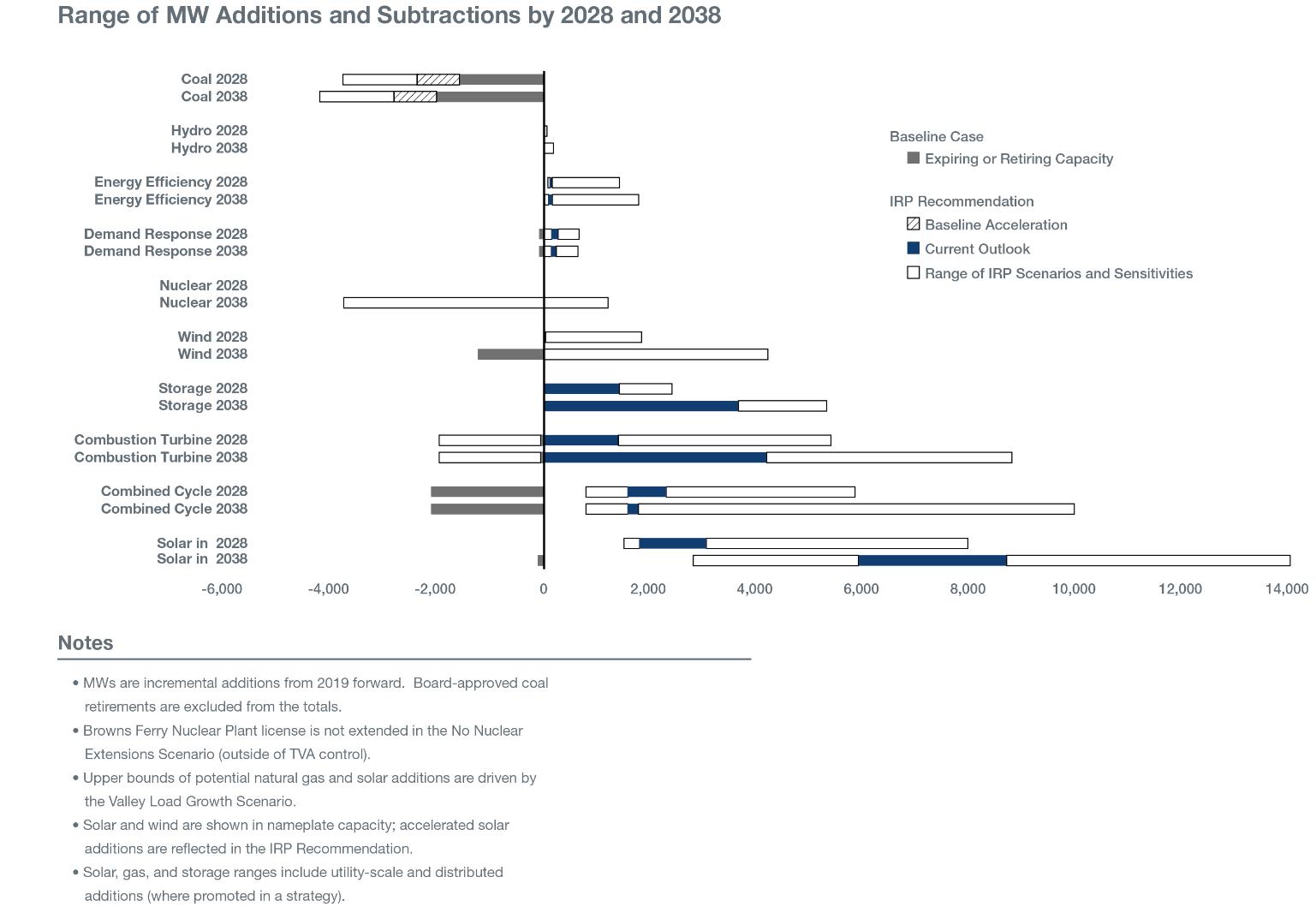
Coal: Continue with announced plans to retire Paradise in 2020 and Bull Run in 2023. Evaluate retirements of up to 2,200 MW of additional coal capacity if costeffective.
Hydro: All portfolios reflect continued investment in the hydro fleet to maintain capacity. Consider additional hydro capacity where feasible.
Energy Efficiency: Achieve savings of up to 1,800 MW by 2028 and up to 2,200 MW by 2038. Work with our local power company partners to expand programs for low-income residents and refine program designs and delivery mechanisms with the goal of lowering total cost.
Demand Response: Add up to 500 MW of demand response by 2038 depending on availability and cost of the resource.
Nuclear: Pursue option for second license renewal of Browns Ferry for an additional 20 years. Continue to evaluate emerging nuclear technologies including Small Modular Reactors as part of technology innovation efforts.
Wind: Existing wind contracts expire in the early 2030s. Consider the addition of up to 1,800 MW of wind by 2028 and up to 4,200 MW by 2038 if cost effective.
Storage: Add up to 2,400 MW of storage by 2028 and up to 5,300 MW by 2038. Additions may be a combination of utility and distributed scale. The trajectory and timing of additions will be highly dependent on the evolution of storage technologies.
Gas Combustion Turbine: Evaluate retirements of up to 2,000 MW of existing combustion turbines if cost effective. Add up to 5,200 MW of combustion turbines
by 2028 and up to 8,600 MW by 2038 if a high level of load growth materializes. Future CT needs are driven by demand for electricity, solar penetration, and evolution of other peaking technologies.
Gas Combined Cycle: Add between 800 and 5,700 MW of combined cycle by 2028 and up to 9,800 MW by 2038 if a high level of load growth materializes. Future CC needs are driven by demand for electricity and gas prices, as well as by solar penetration that tends to drive CT instead of CC additions.
Solar: Add between 1,500 and 8,000 MW of solar by 2028 and up to 14,000 MW by 2038. Additions may be a combination of utility and distributed scale. Future solar needs are driven by pricing, customer demand, and demand for electricity.
TVA’s recommended planning direction affirms its commitment to a diverse and flexible resource portfolio guided by the least-cost system planning mandate. The ranges above provide a general guideline for resource selections. TVA believes meeting its future needs in accordance with the resource technologies and ranges in this recommendation position TVA to continue to deliver low-cost, reliable, and clean power to the people of the Tennessee Valley.
This chapter outlines some of the challenges and next steps TVA faces in implementing the recommendations of the IRP study, and discusses key policy considerations and improvements to modeling and the study process.
In finalizing the IRP and EIS and developing the IRP Recommendation, TVA considered the input received during the comment period. No earlier than 30 days after publication of the notice of availability of the Final IRP/EIS in the Federal Register, the TVA Board of Directors will be asked to make a decision on the IRP Recommendation. After the Board makes a decision, the NEPA process is completed by issuing a Record of Decision that documents the Board’s action and its basis.
The Regional Energy Resource Council (RERC), after reviewing the recommendations in the IRP, offered the following advice to the TVA Board:
1. TVA should monitor federal and state regulations, legal challenges, and industry changes that may alter the broader energy environment and take appropriate actions to mitigate risks to the power system’s reliability and costs.
2. TVA should continue to work with local power companies, directly served customers, and stakeholders to collaborate on Distributed Energy Resources (DER) and distribution planning; build greater visibility into customer needs; and prepare for associated data management. Standardization of cost-effective DER smart technologies will enable the system to efficiently utilize distributed resources.
3. TVA should continue engaging with stakeholders early in any decision process on the site selection for solar, gas power generation, and utility-scale energy storage to avoid land-use conflicts, encourage the
utilization of existing infrastructure assets, and maximize system benefits. In addition, TVA should continue to analyze small-scale, flexible, carbon-free nuclear resources for their potential inclusion in a diverse portfolio.
4. TVA should continue evaluating gaps in data, including customer needs and desires, the speed of technology advancement, locational value, flexibility value, etc., in order to inform and be prepared for future IRPs TVA should also explore advanced data tools to support the analysis.
(Above excerpt from the advice provided by the TVA Regional Energy Resource Council on June 27, 2019. See www.tva.gov/rerc for the full advice statement).
The IRP Recommendation includes significant renewables expansion, introducing operational challenges required to manage intermittency and dynamic loads. Enhanced awareness of the location of renewable resources, both utility and distributed scale, and to weather impacts on solar generation, will become increasingly important. Early experience with battery storage on the system will provide additional insight as to how the various storage use cases might be employed to further support renewables integration and provide economic benefit.
Implementing the recommendations from the IRP will require close cooperation between TVA, local stakeholders, Local Power Company (LPC) partners and Valley electric customers, particularly around deployment of distributed energy resources. TVA is primarily a wholesale power provider and the LPCs have the relationship with most end-use customers. TVA will need to partner with LPCs and other stakeholders in the region to better understand the potential for distributed resources in the Valley and their locational value to inform resource decisions.
The IRP Recommendation also includes more conventional resources, primarily gas-fired, that come with their own implementation challenges in the areas of siting and permitting, both for the units themselves and for the transmission lines and gas pipelines associated with them. TVA has several teams working on various aspects of the siting and permitting work necessary to ensure that when these resources are
needed as part of the generation portfolio, TVA will be better positioned to add them to the resource mix.
The IRP is a resource planning study focused on identifying a target power supply mix for TVA. In the process of developing the cases and reviewing the results with stakeholders, a number of policy-related issues were raised that are outside the scope of the IRP itself, but will need to be considered as we move toward implementation of recommendations from the study.
• Continued evolution of programs that provide flexibility for customer-owned generation
• Evolution of Federal/State energy and environmental policies
• Advancements in customer expectations and requirements for clean energy
• Enhancing low income equity and energy/environmental justice
We also realize that the level of electric rates and job growth are critical concerns for Valley governments, businesses and residents. The IRP uses two specific metrics for the macro-economic impacts of resource strategies. These metrics and underlying analyses provide important information about future revenue requirements that affect future rate levels and will help inform the future direction of TVA’s economic development program. However, none of the strategies had a significantly different impact from the others on the Valley economy. Section 5.5.6 of the EIS provides more information about socioeconomic effects.
The scenarios and strategies evaluated in the IRP provide insights to how TVA’s resource portfolio may need to evolve as the future unfolds. The results also indicate near-term actions that provide benefit across multiple futures. TVA is planning to implement the following near-term actions as part of the IRP:
• Add solar based on economics and to meet customer demand
• Enhance system flexibility to integrate renewables and distributed resources
• Evaluate demonstration battery storage projects to gain operational experience
• Pursue option for license renewal for TVA’s nuclear fleet
• Evaluate engineering end-of-life dates for aging fossil units to inform long-term planning
• Conduct market potential study for energy efficiency and demand response
• Collaborate with states and local stakeholders to address low-income energy efficiency across the Valley
• Collaboratively deploy initiatives to stimulate the local electric vehicle market
• Support development of Distribution Resource Planning for integration into TVA’s planning process
As the future evolves, TVA will monitor key signposts that will guide decisions for the long-term. Signposts relate to key variables that could have a significant influence on the future generation portfolio. Key signposts include:
• Demand for electricity
• Natural gas prices
• Customer expectations
• Regulatory requirements
• Operating costs for existing units
• Solar and wind costs
• Emerging and developmental technologies.
TVA will closely monitor these key drivers related to changing market conditions, more stringent regulations, and technology advancements to inform appropriate actions within the recommended ranges and appropriate timing for initiating the next IRP.
TVA finds considerable value in undertaking an IRP and especially appreciates the input, review and insights of individuals on the IRP Working Group and the RERC. The IRP Working Group and RERC members spent considerable time helping TVA develop a robust plan that meets the criteria outlined in TVA’s objectives. TVA values their involvement and the expertise they provided on behalf of their stakeholders in the development of this IRP.
As with any long-term plan, TVA’s IRP reflects what we know today and can reasonably expect for the coming years. TVA, along with our employees across the Valley, stands ready to carry out its three-part mission around energy, the environment and economic development. In an ever-changing world, TVA will do its best to continue to serve the people of the Tennessee Valley by providing low cost, reliable and clean power in an environmentally responsible manner while promoting economic development across the Valley.


 TENNESSEE VALLEY AUTHORITY
This page intentionally left blank.

AAppendix A - Generating Resource Cost and Performance Estimates
A wide array of new resource options were available in the capacity expansion planning models for selection to meet load growth or fill resource needs. Each resource option has a set of unique characteristics such as capacity, construction time, book life, heat rate, outage rate, capital cost, variable cost and fixed cost. Chapter 5 includes a discussion of the resource options considered in the IRP. An independent third party, Navigant Consulting, Inc. (Navigant), reviewed and compared the TVA planning parameters used in the IRP to other industry sources to ensure the modeled unit characteristics and assumptions were representative of the respective generating technologies. This appendix contains a letter from Navigant (see Section A.2. below) summarizing its benchmarking efforts The appendix also includes TVA’s internal benchmarking efforts (see Section A 3)
A.2.1 Cost and Performance Parameters
Review for the 2019 TVA Integrated Resource Plan (IRP)
July 13, 2018
A.2.1.1 Background
Navigant Consulting, Inc., (“Navigant”) has reviewed and recommended cost and performance parameters for potential new power generation and storage resource alternatives to be considered in the Tennessee Valley Authority (TVA) 2019 Integrated Resource Plan (IRP) (“Resource Estimates”). The work was performed for TVA under purchase order #3890415 (revised) The primary deliverable was a Microsoft Excel workbook summarizing the Resource
Estimates and related assumptions and notes The preliminary draft workbook was delivered on June 20, 2018, and the final workbook was delivered on July 13, 2018.
This report (“Report”) summarizes the work scope, the resources and parameters reviewed, and our primary findings at a high level In performance of this review and Report, we have in part relied on information provided to us by TVA and third parties While we believe this information to be reliable, it has not been independently verified for either accuracy or validity, and no assurances are offered with respect thereto This Report does not represent any endorsement of any particular resource type, nor a guarantee that any resource type is viable or can be ultimately delivered This Report covers the TVA 2019 IRP only. Navigant and its employees are independent contractors providing professional services to TVA and are not officers, employees, or agents of TVA.
As part of the 2019 IRP effort, TVA is identifying and evaluating potential new power generating and storage resources necessary to serve future load
Estimated values for new resource cost and performance parameters are necessary in order to perform generation capacity expansion and dispatch modeling. TVA requires estimated values that are internally consistent and representative of actual values to be observed in practice Parameters include performance and cost for traditional, renewable, and alternative generation technologies, and also for distributed energy and associated storage technologies Estimated values were obtained from several sources including the TVA business units, the Distributed Generation Information Exchange (DGIX), and the IRP project staff itself.
Navigant’s task was to perform a due diligence review of the TVA-provided cost and performance parameter values. This included comparison to credible industry sources, where available, with the objective of determining whether the provided estimates are indicative of what can be expected for the technologies when located in the Tennessee Valley.
The deliverable was a spreadsheet workbook of tables – one for each resource technology – that:
• lists the parameters and associated values provided by TVA,
• lists alternative values as available and relevant, and
• recommends specific Resource Estimates for use in IRP modeling.
Power generation and energy storage resources considered in the review included the following, which represent alternatives for new capacity to serve future load:
• Natural gas-fired generation
o Reciprocating internal combustion engine (RICE)
o Simple cycle combustion turbine
o Combined cycle (with and without Supplemental Duct Firing)
• Coal-fired generation
o Pulverized coal (with and without carbon capture and sequestration)
o Integrated gasification combined cycle (coal) (with and without carbon capture and sequestration)
• Nuclear generation
o Pressurized water reactor (PWR)
o Advanced pressurized water reactor (PWR)
o Small modular reactors
• Energy storage
o Pumped hydro-electric storage
o Battery storage
o Compressed air energy storage (CAES)
• Solar photovoltaic (PV) generation
o Utility scale (both fixed-panel and tracking)
o Commercial rooftop (both small and large scale)
• Wind energy generation
o Located in Midcontinent Integrated System Operator (MISO) or Southwest Power Pool (SPP)
o Onshore within the Tennessee Valley
o Obtained via High Voltage Direct Current (HVDC) transmission
• Biomass energy generation
o Direct combustion at new facility
o Repowering of existing coal facility
Cost and performance parameters vary somewhat according to generating and storage technology, but each technology generally has 11-14 applicable characteristics or parameters for which values were reviewed These include summer net dependable capacity, summer full-load heat rate, build time, annual outage rate, storage efficiency, number of storage hours, storage input demand, book life, plant overnight capital cost, transmission upgrade cost, total overnight capital cost, variable operating & maintenance (O&M) cost, and fixed operating & maintenance cost (both in $ and $/kW-year).
When relevant and reliable industry values for specific parameter values were available, they were utilized for comparison and as a basis for any Resource Estimate. Notes concerning the source and reconciliation of any material differences were provided in the workbook
Navigant provided recommended parameter values and performed direct comparisons with TVA estimates for 272 draft parameters provided by TVA, and provided an additional 22 values for parameters where TVA had not yet formulated a value For about 57 percent of these, the TVA values were determined to be consistent with the recommended values (meaning within 10 percent, measured relative to the original TVA estimate) The remaining 43 percent of the values showed numerical differences of greater than 10 percent, characterized here as “material”. Of the materially different values, over 80 percent were differences greater than 20 percent Some parameters are correlated with others, and one key difference in interpretation or estimation sometimes led to a pattern of differences across parameters
Additionally, variations in underlying classification categories (in cost allocation, for example) can mean that there is some compensation or offsetting in net effects when modeling. Overall, the majority of TVA values were determined to be consistent with recommended values, and otherwise reasonable.
Regarding natural gas-fired generating resources, for the 103 parameter values compared, 45 (44 percent) of the TVA values were consistent with values recommended by Navigant Roughly half of all parameters showed differences of 20 percent or more Systematic material difference between TVA values and recommended values existed in annual outage rates, where the Navigant recommendations were higher across the board Build times recommended by Navigant were generally lower, and overnight capital costs mostly higher. For a given resource, parameter value differences vary in terms of impact, and a number of potentially offsetting differences are evident.
The majority (75 percent) of the 48 coal resource parameters compared were in agreement For the parameters with material differences, there was no systematic pattern, although some differences were noted for plant variable O&M ($/MWh) and fixed O&M ($/kW-year) costs.
For nuclear generation, the vast majority (88 percent) of the 24 parameter values were found to be consistent Total overnight capital costs were 20 percent greater for two reactor types, and variable O&M values were moderately higher than TVA values.
Regarding energy storage, 73 percent of the 26 compared parameter values were materially consistent Each value with a material difference was at least 20 percent different The parameters with such differences included net dependable capacity, book life, total overnight capital cost, variable O&M and fixed O&M costs
Over half (56 percent) all of the solar PV parameter values compared were consistent Net dependable capacity, build time, total overnight capital costs, and fixed O&M costs showed material differences from the Navigant-provided values.
For wind energy, 11 of the 89 parameter values compared (or 39 percent) were consistent, with most of the remaining values showing differences greater than 20 percent Build time, variable O&M and fixed O&M costs were all greater than 20 percent different than TVA values in most cases for the four technology alternatives
Biomass options show consistent parameter values in 44 percent of the comparisons, with material differences in all of the nine remaining values compared. Most of the parameters for repowering existing coal with biomass were at least 20 percent different, reflecting the situational nature of such projects.
On balance for all the generating and storage resources examined, the majority of the proposed TVA parameter values for which comparisons were performed were consistent with recommended values – almost three-fifths of all compared values For those parameters with material differences in values of 10 percent or more, a number of those were to some degree offsetting within a given resource/technology.
The TVA values reviewed were provided in June of 2018, and the summary above relates to recommendations and comparisons based on the values provided at that time Since then, TVA has modified numerous values to be used in its IRP modeling, in part reflecting the outcome of this review. TVA staff were extremely helpful and responsive both in providing supporting information needed in the review/comparison process, and in providing useful feedback and clarification on the draft workbook deliverable and the constituent parameter values It is clear that TVA is striving to fairly represent all of the potential new generating resources in its IRP modeling, thus laying the basis for meaningful IRP modeling of resource expansion alternatives.
When evaluating how to best meet future needs for electricity, TVA optimizes decisions using least-cost planning models. These models require inputs on variables such as capacity amounts, upfront capital
costs, and fuel usage parameters, and many others. The models integrate all the variables for new resources under the various scenarios (i.e., various fuel prices, demand projections, regulatory environments, etc.) to select expansion units that best fit the portfolio needs and requirements in a manner that represents the least system cost
One of the key assumptions that contributes to resource selection is the cost to construct a particular unit. Construction and capital costs are determined from industry experience, vendor information, benchmarking, etc. These costs are presented as Overnight Capital Costs in the table. This is the cost to build the asset and is computed as total dollars divided by the capacity of the unit in kilowatts ($/kW).
Depending on how an asset’s dispatch cost compares to other assets in the fleet, the amount of
energy sourced from an asset may vary greatly over time. For example, when natural gas prices are low, those assets powered with natural gas serve customers with more energy than when natural gas prices are high. A concept that is sometimes used to compare asset costs is Levelized Cost of Energy (LCOE). This measure divides the total cost of an asset (i.e., construction and capital, ongoing maintenance and operating, and dispatch costs which are primarily fuel) by expected output or generation. Because dispatch costs and expected output vary widely across all of the IRP scenarios, LCOE is not a useful metric to benchmark resource costs. A better comparison, and the standard for resource planning, is to compare $/kW installed capital costs. These are the actual inputs to the capacity expansion model and the costs benchmarked by TVA’s independent thirdparty contractor.
TVA engaged an independent third party, Navigant Consulting, Inc. (Navigant), to review cost and
performance assumptions proposed for use in the 2019 IRP. Navigant evaluated TVA’s assumptions for various unit types along with assumptions for distributed resources in a collaborative effort with stakeholders. This independent assessment found
that the majority of assumptions proposed for the study were consistent with typical values used in the industry. Many of the remaining assumptions were modified, based on Navigant’s recommendations, prior to running the IRP cases. The data in the table presented in the preceding section reflects adjustments recommended by Navigant.
TVA also prepared a comparison of its capital cost assumptions from the IRP study to a recent Lazard
report, EIA data and other utility IRPs to further verify the reasonableness of TVA’s assumptions. This comparison chart, Figure A-1, shows how TVA’s assumptions on capital costs compare to those recently published sources. The cost comparisons are generally consistent given that the majority of the data points are based on national averages and TVA’s costs are specific to the TVA system and reflect recent project experience and quotes
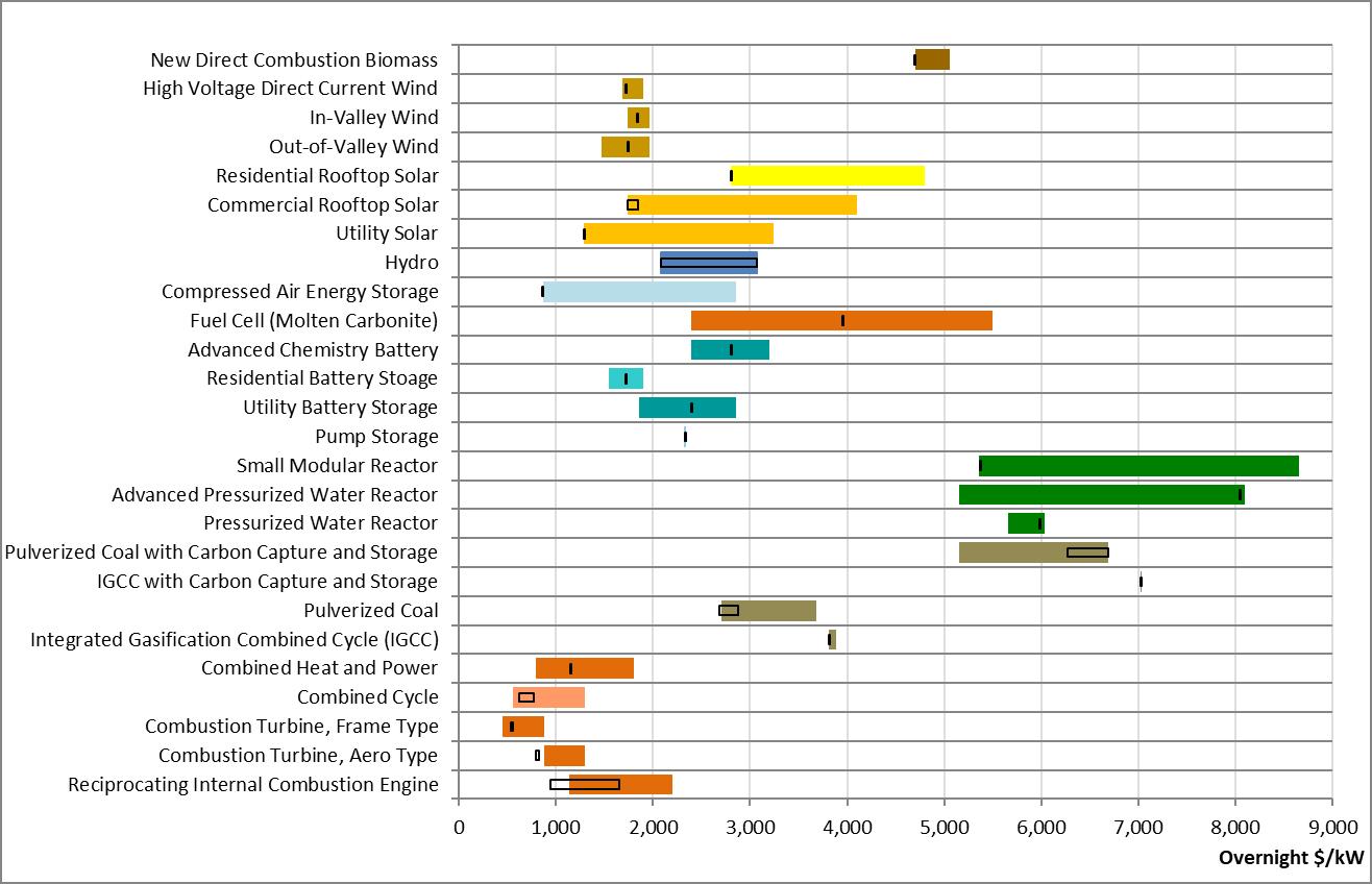
Wind and solar resources have unique operating characteristics that are different from thermal and other more traditional resources. To properly account for the contribution from these intermittent resources, the energy contribution is represented using hourly energy profiles that are imported into the model, and
the seasonal capacity of these resources is represented by a computed Net Dependable Capacity (NDC) value. The annual capacity factor of the hourly energy profiles is also computed to ensure the total amount of energy is comparable to industry benchmark sources. This appendix discusses the methodology TVA used to determine both the energy profiles and NDC values for wind and solar options that are considered in the IRP.
Generation from wind is weather and location dependent and not dispatchable like more conventional resources. Therefore, utilities need to develop a reasonable representation of the output from wind for use in long-range planning models. This “wind shape” is based on actual data collected from specific sites, or modeled data using wind turbine design assumptions.
TVA uses a combination of data from 3TIER, a thirdparty company specializing in renewable energy assessment and forecasting, and data from TVA wind PPAs to develop the planning assumptions around wind shape and capacity factor for use in the IRP. A “typical week” hourly shape for each month was developed by 3TIER for each wind option. From these shapes, the amount of energy produced can be determined and a capacity factor computed (actual generation expressed as a percentage of maximum possible generation).
TVA used actual results from its wind contracts (1,200 MW in Oklahoma, Illinois, Kansas and Iowa), simulated and actual data for the in-Valley sites, and proposals for various projects to determine the capacity factors for the wind resources options included in the IRP. Since each of the options originates from different regions, TVA used a regionspecific estimate for annual capacity factors. For modeling purposes, TVA assumed the MISO and SPP option had a 40 percent capacity factor, the HVDC option originating from Oklahoma had a 55 percent capacity factor, and the in-Valley option had a 30 percent capacity factor
The HVDC project has a 55 percent annual capacity factor due to the availability of wind in Oklahoma and the newer technology of the wind turbines, which were assumed to be GE 1.7-100 wind turbines at a height of 80 meters. This capacity factor is much higher than TVA’s existing wind contracts in other locations. Figure A-2 shows the range of capacity factors:
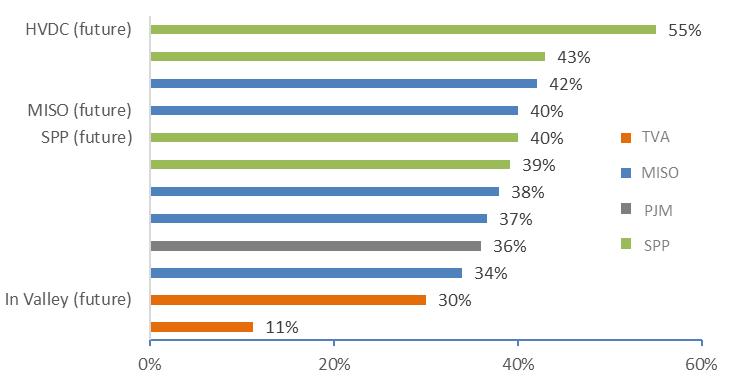
Planners must determine how much wind generation is likely at the summer and winter peak hours so that appropriate Net Dependable Capacity (NDC) credit can be given to wind resources when computing the capacity/load balance to determine if the required reserve margins have been met in a given year. The NDC is applied to the nameplate capacity and is used by the expansion model as a wind resource’s contribution toward meeting reserve margin requirements
For this IRP study, TVA used 39 years of simulated and actual hourly wind data ranging from 1980 to
2018 This 3TIER study simulated data was not updated for this IRP as material changes in historical and simulated wind data were not expected. The wind generation was based on simulation of TVA’s existing wind contracts in MISO, SPP, and PJM as well as a site in Kansas near the proposed HVDC site TVA and 3TIER data were used to assess the long-term variability of the wind for each site in a retrospective analysis of historical wind speed and power. These data points were derived from a mesoscale Numerical Weather Prediction (NWP) model that was statistically calibrated to match the observed data during the measurement period at the height of the towers. An example of the variability of the wind net power is shown in Figure A-3.
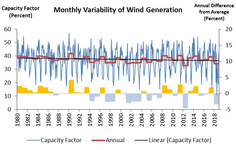
NDC was calculated as 14 and 31 percent for summer and winter, respectively, based on a portfolio view of all current wind contracts to capture the diversity of location across the different states of the region (i.e., Oklahoma, Kansas, Illinois, Iowa). These NDC values were used for all wind options. Further detail on how wind NDC values were calculated is
included in the Intermittent Resources Study section of Appendix D.
Because specific sites of future wind in MISO, SPP or In-Valley is unknown, it would be inappropriate to assume a different NDC at this time A more specific NDC would be incorporated into the wind portfolio NDC calculation once specific sites are known. TVA
did not consider over-subscription contracts where transmission is limited to a level below the nameplate rating of the wind capacity which tends to improve both the annual capacity factor and the NDC rating. The costs associated with the wind projects modeled in the IRP do not reflect oversubscription. In TVA’s experience with several existing wind contracts, this over-subscription provision is negotiated through the terms and costs of a particular contract and is not easily comparable to industry benchmarks
Similar to wind, solar resources are also weather and location dependent. Modeling of solar options in the IRP proceeds in a similar fashion to wind, and
requires determination of solar shapes, capacity factors and NDC values. Solar data for the 2015 IRP was provided by members of the TVRIX stakeholder group who commissioned Clean Power Research (CPR) to provide TVA with the solar energy profiles for 26 sites across the Tennessee Valley shown in the map below. CPR provided SolarAnywhere® data for 15 years (1998-2013) of consistent, validated, timeseries irradiance measurements that provided the historical basis for the NDC, capacity factors and hourly energy patterns This data was collected for the 2015 IRP and was not updated as material changes were not expected. However, TVA also incorporated capacity factors and hourly generation patterns from TVA solar PPAs to inform assumptions in the 2019 IRP.
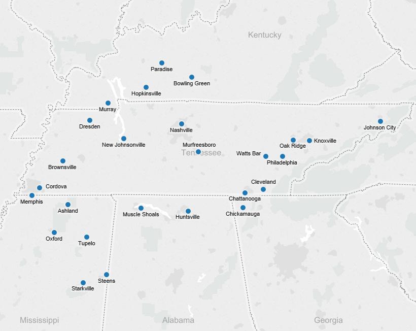
Using the data supplied through CPR as well as PPA data, TVA determined that annual capacity factors are
The determination of the NDC for solar resources utilizes the same process as described for wind
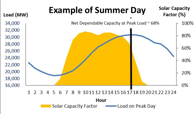
In the summer, TVA normally has a peak load at 5:00 p.m. CST, but can also see a peak load between the hours of 2:00 p.m. and 6:00 p.m. CST. The 25th percentile of solar generation of those hours would occur at 5:00 p.m. or 6:00 p.m. CST as the sun is
20 percent for the fixed axis and 23 percent for the single-axis tracking option. The monthly capacity factors vary as shown in the following chart.
resources The figure below shows the range of NDC values for solar fixed-axis systems computed using the CPR and TVA PPA data.
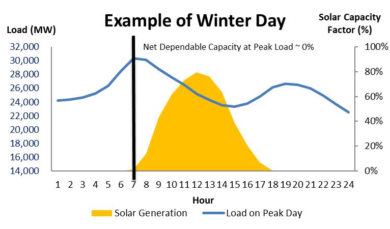
setting. Therefore, the summer NDC was set at 50 percent for fixed axis at all scales. The utility tracking option has a 68 percent summer NDC. All solar options have a zero percent NDC during the winter, since TVA’s winter peaks normally occur around 7:00
a.m. CST when solar is not available. Further detail on how solar NDC values were calculated is included in the Intermittent Resources Study section of Appendix D.
Appendix B - Programmatic Resource Methodology
BAppendix BProgrammatic Resource Methodology
TVA utilizes a diverse portfolio of energy resource options to provide electric power service at the lowest feasible rate, including the use of programmatic
resources related to demand response (DR), energy efficiency (EE) and beneficial electrification (BE). Collectively, these will be referred to as DER programs. These offerings can include incentive programs, pricing products and educational efforts to encourage informed consumer choice. Programs are offered under the EnergyRight® Solutions (ERS) brand and span residential, commercial and industrial sectors. Over the years, TVA programs changed to suit the evolving energy landscape, as depicted in Figure B-1.
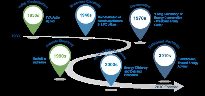
For over thirty years, TVA offered DR programs that incent commercial and industrial customers to reduce loads during periods of high demand. Since the mid 2000s, TVA facilitated EE programs that incent energy efficiency across all sectors. Currently, TVA also offers BE programs that help customers reduce overall energy costs, emissions, or both.
DR programs reduce system load at peak hours and potentially offset or delay the need for more expensive peaking generation or power purchases. Various programs provide incentives or price structure changes to commercial and industrial customers in exchange for them suspending a portion of their load during peak periods. These programs act as a zero emissions resource to the TVA system.
EE programs target efficiency upgrades and improvements to reduce system load across many hours. Programs provide incentives or educational opportunities to consumers to spur efficiency improvements in their homes or businesses above and beyond current codes and standards. By reducing inefficient energy use, EE programs help lower fuel costs and decrease emissions. As U.S. Department of Energy (DOE) codes and standards have increased and energy efficiency has taken hold in most market sectors and reduced electricity demand, TVA has reduced EE incentives. However there is opportunity to reduce energy burden within the Low Income residential sector, which has more limited opportunity to adopt energy efficiency technologies In 2016, TVA initiated an Energy Efficiency Information Exchange stakeholder group to work together to launch a sustainable and equitable
low-income energy efficiency and education model in the Valley In 2018, TVA launched a Low Income EE pilot program focused on education and outreach coupled with incentives for home upgrades leveraging matching funds from federal programs, LPCs and local communities.
BE programs promote adoption of smart energy technologies across all sectors. Current BE programs incent commercial and industrial customers to utilize equipment powered by electric rather than other conventional sources and incent residential customers to use electric sources for space conditioning and water heating. These programs have the potential to reduce fuel costs and/or societal emissions as compared with individual gas and diesel powered appliances and equipment.
To model DER program options for the IRP, TVA leveraged experience and historical data to estimate load changes and costs of potential DR, EE and BE
programs. TVA uses a third-party provider (DNV-GL) to evaluate, measure and verify program impacts, and DNV-GL also provides insights on the potential impacts of new programs based on their experience working with TVA and other utilities. Additionally, TVA conducts a Residential Saturation Survey and a Business & Industry Saturation Survey every other year to understand market depth and potential reach of programmatic efforts, which vary from region to region. TVA is also an active participant in and member of multiple industry trade organizations that specialize in energy programs, including eSource, Association of Energy Services Professionals, and others.
Because IRP strategies explore various levels of DER program incentives, it was necessary to model options for selection. As TVA utilizes a combination of education and monetary incentives to encourage greater levels of program participation, a three-tiered approach was taken to develop program offerings for selection (Figure B-2).
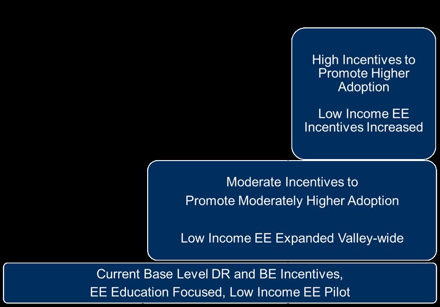
Tier 1 programs reflect current incentive levels for DR and BE programs, and an emphasis on education with no or low monetary incentives for EE programs beyond the Low Income EE pilot program. Tier 2 programs build on Tier 1 by providing a moderately high monetary incentive for all programs equal to 50 percent of the marginal cost of a comparable generating unit in each scenario. While resources can provide energy and capacity, IRP modeling takes a simplified approach to use marginal energy cost for EE and BE and marginal capacity cost is used for DR, aligning to the primary role of each resource Tier 3 programs further build on Tiers 1 and 2 by providing a high monetary incentive equal to 100 percent of the marginal cost of a comparable generating unit. Tier design takes into account the market depth potential at each level of incentive.
The incentive level effectively reduces the price of a given program in a given strategy. The model is then
given the freedom to select the programs and other resources in order to create the lowest cost system portfolio. Low Income EE programs are the exception, as they are enforced in the model at levels applicable in each strategy due to the high cost of these programs.
Strategy design applies a base, moderate or high level of promotion aligned to each strategy narrative A base level of promotion includes Tier 1 incentives for each program, moderate level includes Tier 1 and 2 incentives, and high level includes Tiers 1, 2 and 3 incentives Figure B-3 depicts the base, moderate or high promotion for each DER program resource type applicable in each strategy.
Low Income EE programs are treated as required resources, with applicable tiers enforced in the model according to each strategy. While all strategies include programs from Low Income EE Tier 1, the Promote DER strategy also includes Tier 2, and the Promote Efficient Load Shape strategy also includes Tiers 2 and 3.
B.1.3.1 Demand Response (DR)
DR resources reduce system load at peak hours. Figure B-4 illustrates summer and winter load shapes and typical peak or near-peak demand hours around which DR is most likely to be called upon for economic or reliability reasons
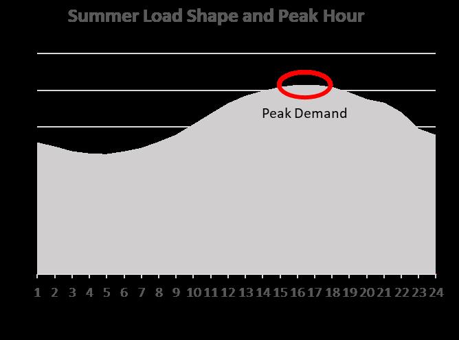
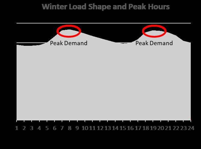
Current TVA DR programs include the Interruptible Power Program (IP), Peak Power Partners, Voltage Optimization, and Instantaneous Response. The 2019 IRP assumes existing programs will continue through their respective program lives with pricing generally aligned to the projected carrying cost of a natural gas combustion turbine (CT)
IP is TVA’s largest DR segment and includes the IP30 and IP5 sub-programs. Large industrial customers allow TVA to call on them to reduce their electric load during peak hours when supply is tight or costly, in exchange for a pricing reduction. When called upon, participants in the IP30 program are given 30 minutes’ notice to reduce their load to a specified amount. The IP30 program may be used for economic or system reliability reasons. Participants in the IP5 program are given 5 minutes’ notice to reduce their load to a specified amount. The IP5 program can only be used for system reliability. IP currently supplies about 1,500 MW of load reduction.
Peak Power Partners utilizes third-party program administrators to aggregate smaller commercial and industrial customers to meet load reduction targets. While similar in concept to IP, Peak Power Partners is smaller and currently supplies about 100 MW of net load reduction. Contracts with program administrators must periodically be renewed, and the IRP baseline case assumes a renewal of an aggregated DR program at the cost of a comparable gas CT unit.
The Voltage Optimization program works in partnership with LPCs to lower the voltage on their
respective systems to the lower half of the acceptable voltage range. This program currently supplies about 200 MW in load reduction and can be scheduled dayahead or as part of a longer-term conservation effort. Current Voltage Optimization programs extend into the early to mid 2020s.
In this IRP, we are also including DR program options for the residential sector. Programs for aggregated control of residential space conditioning and water heating have been modeled for selection.
EE programs span all customer segments and focus on reducing electrical consumption overall. Since temperature is the largest driver of peak loads, particularly in the residential sector, many EE programs focus on space conditioning (HVAC) and weatherization improvements. Programs may also include more efficient lighting, variable frequency drives, and other custom options tailored to a specific industry.
The eScore technology platform is the cornerstone for the residential segment. The eScore system is currently being leveraged as a tool to educate the end-use consumer, as well as build and reinforce consumer trust Consumers can use the platform to ensure their contractor has been trained and approved and their installation has been performed to program standards. The flexibility remains to include incentives where they may apply in the future. Residential customers can also use eScore to set up appointments for home efficiency evaluations.
Following the home inspection, the customer will receive a detailed report including an efficiency score (1-10), pictures of problem areas, and recommendations. Contractor search and validation enables customers to find contractors who have been vetted and trained by TVA, providing peace of mind when selecting a contractor for home improvements. The Tier 2 and 3 offerings, mentioned in section B.1.1 above, would reintroduce incentives to the eScore program. These incentives are generally in the form of customer rebates following verification that certain home efficiency projects were completed by TVAvetted contractors. In the past, these rebates included window upgrades, HVAC replacements and additional insulation.
An important aspect of residential EE offerings are TVA’s Low Income EE programs. Since 2009, TVA has partnered with the state of Tennessee’s Weatherization Assistance Program (TN WAP) to provide home energy audit and upgrade services to families with incomes less than or equal to 200 percent of the federal poverty level for the household size. The DOE provides funding for this program, which is then administered locally by the state of Tennessee. TVA continues to provide administrative and technical support to TN WAP to ensure the state takes advantage of all available DOE funds. TVA’s Home Uplift initiative, currently in pilot phase, seeks to augment TN WAP by working with LPCs and local communities to create a sustainable program aimed at making weatherization improvements in low income households. TVA contributes about 50 percent of the funds, with the remainder contributed by LPCs, local governments and non-profit agencies. Tier 1 includes Low Income EE education and outreach programs and Home Uplift at the pilot program level. Tier 2 includes all programmatic elements from Tier 1 and additionally expands Home Uplift from pilot phase to a Valley-wide program under the same matching concept. TVA would provide seed
money necessary to begin Home Uplift programs with LPCs across the Valley, contingent on matching funds. Tier 3 includes all programmatic elements from Tiers 1 and 2 and, additionally, expands Home Uplift by finding grant sources and partnering agencies and matching that additional level of funding.
Commercial and industrial (C&I) EE programs include some standard rebates, but focus more on customized solutions. Tier 1 continues support of Strategic Energy Management (SEM), which provides a forum to allow companies to work together to identify common energy efficiency challenges and develop common solutions. An example solution may involve a company discussing the advantages and lessons learned from installing smart thermostats at their facility. SEM has traditionally focused on the industrial sector, but is being expanded to include the commercial sector. Tier 2 and 3 C&I offerings include incentives. Example programs include LED lighting retrofits, variable frequency drives, or HVAC upgrades. Industrial projects tend to be highly customized based on a given customer’s use case. For custom projects, the customer would provide TVA with a proposed plan, obtain approval for the plan, implement improvements, and receive rebates following verification for completed projects.
The impact of the EE programs on TVA’s load will vary by customer segment, season, and time of day (Figure B-5). Residential EE programs have the greatest impact in late afternoon hours and early winter morning hours when residents are returning home from work and school or preparing for the day Commercial EE load impacts are typically higher during traditional business hours. Due to round the clock shifts, industrial EE impacts are generally more consistent throughout all hours. Sector impacts also vary depending on whether a program targets HVAC, lighting, other equipment, or a combination of these aspects
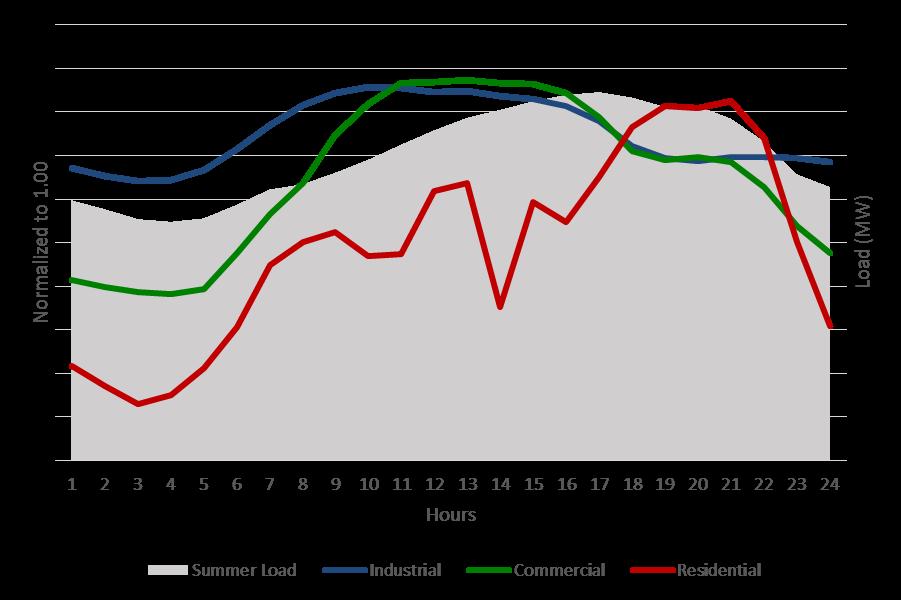
Consumer preference, as well as increased DOE codes and standards, have resulted in a nearly flat load forecast across the TVA region over the planning horizon. Consumers across customer segments see the benefits of replacing older lighting solutions with more efficient LEDs, while appliances such as HVAC and refrigeration systems continue to improve efficiencies. As less efficient technologies continue to age and go out of use, the percentage of electrical load they displace will continue to grow. While TVA’s past EE programs also had an impact on efficiency efforts, these impacts have been greatly surpassed
by the market-driven effects. Figure B-6 depicts the impacts that market-driven and TVA programmatic EE has had on TVA’s weather-normal system load since 2007, along with the forecasts included in the Current Outlook scenario. The 2019 IRP EE expansion options are available starting in year 2020; therefore, Figure B-6 only includes impacts from TVA programmatic EE installations from years 2007-2020 that are already included in TVA’s business plan EE expansion included in the results for each portfolio would be in addition to the impacts included in this chart.
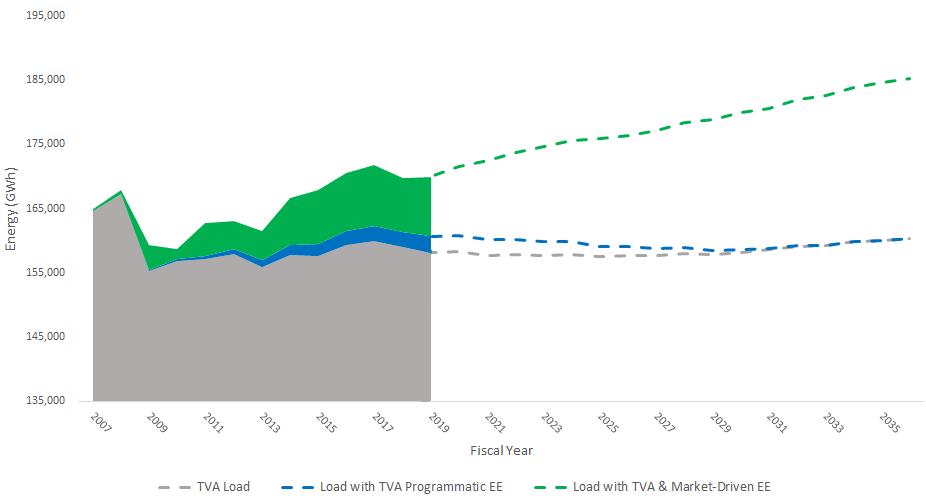
B.1.5
BE programs span all customer segments and focus on adoption of smart energy technologies. Residential programs encourage the use of electric or dual fuel space conditioning and appliances. BE programs incent commercial and industrial customers to utilize equipment powered by electricity, rather than other conventional sources.
The eScore platform is also being leveraged to deliver residential BE programs. Tier 1 includes education, as well as rebates for residential customers switching from gas to electric or dual fuel. Programs cover dual fuel heat pumps, air source heat pumps, mini-split units, and conventional electric water heaters. Additionally, the residential segment includes a new homes program which provides rebates to builders who install electric HVAC, water heaters, and appliances in new construction. Tiers 2 and 3 build on these existing programs with additional marketing and increasing levels of rebates.
Commercial and industrial (C&I) BE programs are generally more customized than residential offerings. C&I incentives may include rebates to encourage the use of electric forklifts or electric options for food service and other equipment. TVA works with industrial customers to develop solutions to modify processes to reduce customer cost while also benefitting TVA’s overall system load shape.
The BE impact to TVA’s load will vary based upon customer segment (Figure B-7). Residential and commercial BE programs will have the greatest relative impact during the day, when Valley residents are awake and businesses are open Due to energy intensity and round-the-clock shifts, industrial BE programs tend to have a higher and more consistent impact across all hours and the biggest impact for dollars spent.
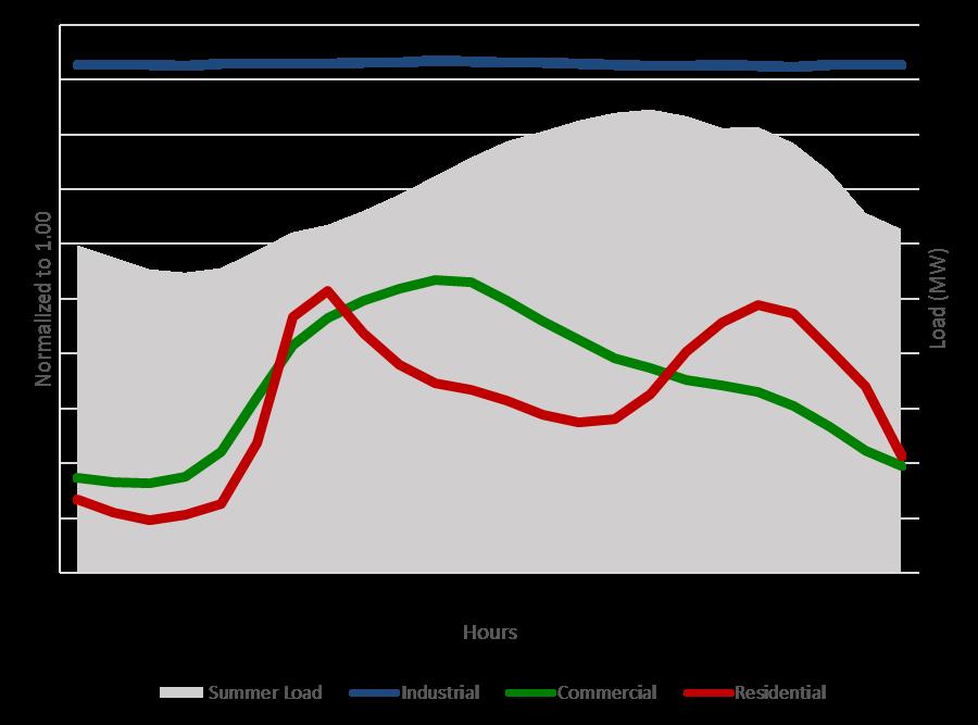
For DER programs to be offered for selection in the optimization model, certain characteristics must be defined that are comparable to conventional supply side resources.
Conventional supply side resources have the following characteristics:
• Capacity and energy - typically a known size in MW and MWh, respectively
• Installation cost – typically non-site specific $/kW
• Construction lead time – years to build from initial project consideration
• Operational characteristics – heat rate (fuel efficiency), capacity factor, etc.
• Service Life – years
DER program characteristics must be developed that are comparable to supply side resources. Figure B-8 compares supply side and DER program unit characteristics that feed the capacity planning model.
*Conventional Resources could include nuclear, coal, gas, hydro, etc.
Similar operational characteristics of each sector program were developed for all tiers, including additional costs that would be incurred to expand delivery system infrastructures and encourage greater participation. Tier 1 programs generally represent costs for platform infrastructure and business as usual, and as such, have known costs. The steps in cost for Tiers 2 and 3 are similar to a supply stack concept, where programs with more potential are lower cost programs and programs with less potential are higher cost programs. As market depth is exhausted from the lower cost programs, the optimization model moves up the supply stack to the next lowest cost program. The exception is the Low
Income EE program for which volumes are enforced at base, moderate and high levels as appropriate, before applying least-cost optimization in each strategy. Figure B-9 illustrates the range of costs for each segment and programmatic DER resource type. The ranges shown span the costs of all three tiers. Tier 1 typically includes some initial startup and administration costs that can be leveraged in other tiers, whereas Tiers 2 and 3 have higher incentives in order to attract higher participation. Finally, commercial and industrial programs are typically lower cost on a $/MWh basis compared to residential due to project economies of scale
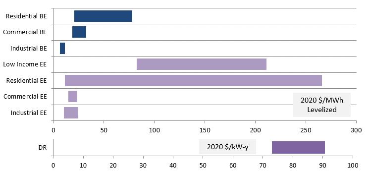
Much like supply side counterparts, programmatic DER programs also have operational-like limits on the maximum energy reductions or additions. The limits are driven by program development, customer awareness, market penetration, participant acquisition and many other customer and market factors. TVA is able to calculate an estimated participation rate for each program tier using historical data, based on the
level of incentives provided. The optimization model will add the full quantity from the next available tier for a given programmatic DER segment if it determines that program to be the least cost resource. New Programmatic DER resources are available for selection in the model starting in 2020. Details for the individually modeled programs are shown in Figure B10
* While tiers are generally shown as incremental, Low Income EE tiers are shown as cumulative due to program structure (i.e. Tier 2 includes Tier 1 and Tier 2 impacts)
^ Capacity impacts for each program tier are shown at TVA's system peak for both summer and winter
As in the 2015 IRP, EE is being treated as a selectable resource. We have continued to innovate by adding selectable DR and BE resource options to the mix. DER programs are modeled in a manner consistent with how conventional supply side resources are modeled (i.e. nuclear, coal, gas, hydro, etc.), including a defined energy pattern (i.e. the load shape) similar to a solar resource. The three-tiered approach (see Figure B-2) builds and improves upon the block method used in the last IRP by more specifically defining program offerings and associated impacts and costs.
This allows TVA to model selectable DR, EE and BE resources for full optimization. EE and BE programs are non-dispatchable and operate similarly to other non-dispatchable generation resources in that system operators cannot directly control impacts based on system needs. There are no variable operations and maintenance (VOM) costs or emissions penalty (CO2 costs) for non-dispatchable resources. Key input parameters are monthly avoided capacity, $/kW (cost divided by summer peak kW), and an hourly energy pattern.
Increased experience and continuous improvement in the design and implementation of programmatic DER since the 2015 IRP gives program designers a better understanding of the costs, availability and load impacts of the programs modeled. Therefore, TVA is not applying the Planning Factor Adjustment that was present in the 2015 IRP to account for certain risks.
EE and DR programs have two basic impacts that are relevant to planners, with EE having a larger energy impact and DR having a larger capacity impact:
• Avoided energy calculation – Energy not consumed means fuel not burned, resulting in savings in variable costs. Further, since program impacts are realized at the consumer meter, they also avoid applicable transmission and distribution (thermal) losses
which can average up to 6.5 percent by the time energy reaches an end user.
• Avoided capacity calculation – Capacity is avoided, because reduced electricity demand translates into reduced need for incremental capacity additions.
BE programs take the same impacts into account with the potential to increase rather than avoid costs, ideally in a manner beneficial to overall system load shape, customer costs and net emissions:
• Increased energy calculation – Additional energy consumed means additional fuel burned, ideally at times when the TVA and LPC systems can efficiently supply that energy. Some programs may eventually require transmission or distribution system upgrades.
• Increased capacity calculation – Capacity may be added when the benefits of adding load offset the cost of incremental capacity additions
Using EE and BE program design parameters, hourly demand profiles are developed via engineering models and then calibrated through program evaluation. Inputs to the models include occupancy/utilization profiles, building characteristics and weather data. The model provides an 8,760 hourly profile of a “before” end use shape and an “after” efficient end use shape that are subtracted to derive the program impact shape. That shape is then regressed on weather and calendar variables, revealing the relationship between temperature, day of week, season, etc. The model is then forecast forward using TVA weather and load forecast as inputs. The final result is an hourly net forecast synched to the TVA load forecast.
For supply side resources in the IRP, unit performance is not expected to be 100 percent. This delivery risk is captured in an outage rate for the unit. There is not a comparable outage rate for the modeled programmatic DER; rather, the modeling approach assumes programs to be operationally available 100 percent of the time. Efficiency and electrification are dependent on variables such as
equipment reliability and service life, operating conditions, etc., that would impact operability similar to an outage rate. In addition to outage rates, there are other potential uncertainties for DER programs (as compared to supply side resources) in that costs such as CO2 emissions penalty, fuel cost uncertainty, project cost contingencies and cost escalation uncertainties are not captured.
Measure
Fixed Shape
EE and BE impacts manifest themselves in load, as do other variables such as
Programmatic DER introduces some uncertainties around design and delivery (Figure B-11) that are unique relative to other resources. Design uncertainty is introduced by the creation of programs today that may have different costs, lifespans or load shape impacts over time. Delivery uncertainty exists around claimed versus evaluated measures, the ability to deliver and implement programs though TVA’s 154 different local power companies, and risk around EE deliveries relative to future codes and standards.
Stochastic analysis, discussed earlier in the IRP document, will evaluate risks of load uncertainty driven by DER programs and many other factors.
This page intentionally left blank.
Appendix C - Distributed Generation Methodology
CAppendix C - Distributed Generation Methodology
TVA utilizes a diverse portfolio of energy resource options in order to provide electric power service at the lowest feasible rate. Traditionally, utility companies generated electricity at large scale and delivered all of the power needs of end consumers. Recent technology advancements and consumer preference have led to increased interest in distributed generation (DG). The 2019 IRP focuses on three main sources of distributed generation: solar, solar with storage, and combined heat and power (CHP).
At TVA, DG was introduced through the Dispersed Power Program (DPP) in 1981 to comply with provisions of the Public Utility Regulatory Policies Act of 1978 (PURPA). DPP’s primary aim was to allow commercial and industrial customers the ability to sell back excess generation to the grid. In 2003, TVA introduced a small-scale distributed generation program, most recently known as Green Power
Step 1
2
Due to decreasing prices and increasing consumer demand for energy choice, distributed generation is expected to continue to grow. TVA system planners and forecasters, with input from TVA stakeholders, worked together to determine likely levels of distributed solar, battery and CHP penetration across the various scenarios modeled. These scenarios include levels of DG that would naturally occur in the
Providers. Finally, TVA’s mid-scale programs, such as the Flexibility Research Project (FRP) pilot, facilitate LPC community solar offerings, a more convenient and cost-effective alternative to rooftop installations for consumers to support distributed renewable generation.
For the 2019 IRP, TVA developed an innovative way to model adoption of distributed generation technologies. First, the base level of market penetration for each distributed resource type is calculated based on assumptions present in the various scenarios. Next, the level of incentives certain strategies will apply to reduce payback on investment is determined. Then, an adoption curve approach is used to simulate higher penetration levels achieved through improved economics. Next, these new penetration levels are enforced in the capacity expansion model as a required resource. Finally, the capacity planning model optimizes the remainder of the resource portfolio in a least cost manner. This new DG methodology allows TVA to gain insights into the roles DG could have on the TVA system under a variety of different future states. The individual steps are discussed in greater detail in the following sections.
penetration for each scenario by resource type, prior to any additional TVA incentives.
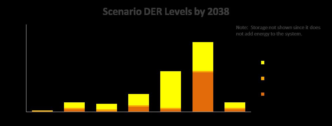
For further information on how unique assumptions around DG were developed for each scenario, see Appendix E: Scenario Design. As each strategy is applied in a scenario, the base level of adoption in each scenario sets the baseline comparison. There will be relatively less opportunity to increase adoption in scenarios where DG penetration is already high before applying the strategic incentive, due to market depth limitations.
As part of Strategy D, Promote Efficient Load Shape, a time-of-use rate structure is modeled to incent
owners of electric vehicles and distributed batteries to charge these devices at economically efficient times. The TVA system experiences different peak hours, depending on the season. In the summer, the system peaks in the late afternoon. Winter peaks typically occur early in the morning, with a near-peak early in the evening. On-peak hours require TVA to use more expensive peaking generation sources, raising system costs. TVA developed a modeling approach to evaluate the impact of a time-of-use rate structure that strongly promotes EV charging in super off-peak (i.e., hours of minimum load) and off-peak hours. The modeled approach, shown in Figure C-3, is similar to Georgia Power’s Plug-in Electric program with modifications to match TVA’s unique system peaks.

The impact of a time-of-use rate structure would be felt in electricity demand. Therefore, TVA forecasters developed a modified load forecast to simulate the modified load shapes resulting from a time-of-use rate incentive for EV and battery charging. This modified load forecast was only used when applying Strategy
D.
Except for the Base Case, all strategies used in the IRP promote increased DG adoption. Monetary incentives are used to increase penetration levels by reducing the payback period for a given resource. While resources can provide energy and capacity, IRP modeling takes a simplified approach to use
marginal energy cost for most incentives, including for DG. A base incentive level aligns to no additional incentive beyond existing programs. Moderate incentives for distributed solar and CHP are modeled at 50 percent of marginal energy cost, whereas distributed storage is incented by matching 10 percent of the distributed solar capacity. As an example, for every 100 MW of distributed solar, an additional 10 MW of battery storage is included. Finally, high incentives for distributed solar and CHP are modeled at 100 percent of marginal energy cost, and distributed storage is incented by matching 25 percent of the distributed solar capacity. Distributed storage is handled differently from other resource types, as the technology is rapidly evolving and there was a desire to understand its impact in combination with distributed solar.
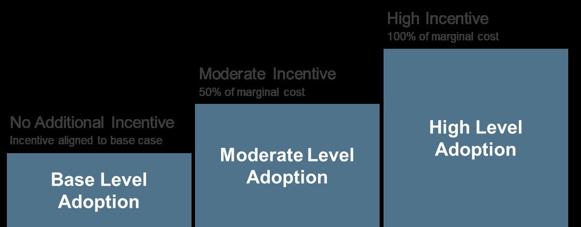
Applying various levels of incentives across the strategies allows TVA to test the impacts of increased DG penetration. The matrix shown in Figure C.5
shows the incentive levels by DG resource type for each strategy.
For additional information on rationale behind incentive levels for DG in each strategy, see Appendix F: Strategy Design.
Base, moderate, and high penetration levels for DG resources were determined using an adoption curve approach. The approach used is similar to National Renewable Energy Laboratory’s (NREL) Distributed Market Demand Model, which simulates potential adoption of a given resource as a function of payback
period. Factors specific to each scenario and strategy combination were fed into a TVA-developed DG model to create a unique adoption level for each resource for the 20-year planning horizon.
The key elements in NREL’s model are the payback period, maximum market share and adoption curve
The payback period determines the maximum market share, or depth, for a DG technology. It also influences the pace of adoption. The concept behind the NREL model is illustrated in Figure C.6, and a simplified application of this model in the IRP is further explained in the following sections.
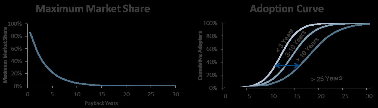
A key element in the model is the payback period, which is simply the number of years required for a consumer to recoup the upfront costs of an investment. Ignoring discount rates, an example project requiring an upfront capital investment of $10,000 that saves a net $1,000/year will have a payback period of 10 years. The lower the payback, the greater the market depth, as more Valley residents see value in adopting a particular technology. Even with an acceptable payback, not all consumers will adopt the technology at the same time. This occurs for a variety of reasons. Some consumers are more comfortable using new technologies than others and are likely to adopt sooner, while others will wait. Also, a consumer must have access to the capital required to cover the initial costs of the technology investment. Even with the necessary capital, whether or when a consumer purchases a technology depends on competing uses for the funds and other practical considerations. All these factors impact the pace of DG adoption, which happens over the course of years and is generally faster with quicker paybacks.
There are two primary components in calculating payback for a DG investment – electricity bill savings and DG investment. To estimate electricity bill
savings, forecasts for residential and commercial average effective rates were applied to the average annual energy output of a DG system. Next, it was necessary to estimate projected prices for distributed solar, storage and CHP systems. Pricing information for DG resources was derived from a variety of sources, both internal and external to TVA.
Distributed solar prices were obtained from Navigant Consulting, with references to NREL studies. These studies contained historical solar prices for all customer segments, up to 2017. These prices were then projected into the future, using pricing improvements TVA has seen in recent solar requests for information and proposals as a directional guide for near-term movements.
Distributed battery prices, including installation costs, were derived from market prices for Tesla Powerwall 2 systems. These prices were projected into the future using IEEE mid-range projections as a directional guide. CHP prices were derived from a combination of information sourced from the Southeast CHP Technical Assistance Partnership and internal TVA surveys of universities, hospitals and commercial entities. Escalation rates for all DG resources can vary by scenario, driven by assumptions around tax policy and pace of technology advancement. Figure C.7 shows assumptions for distributed solar and storage cost projections.
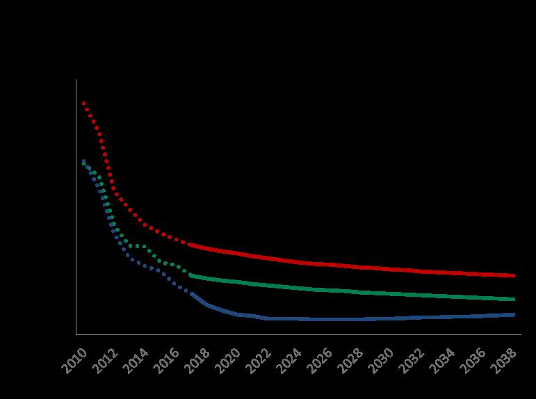
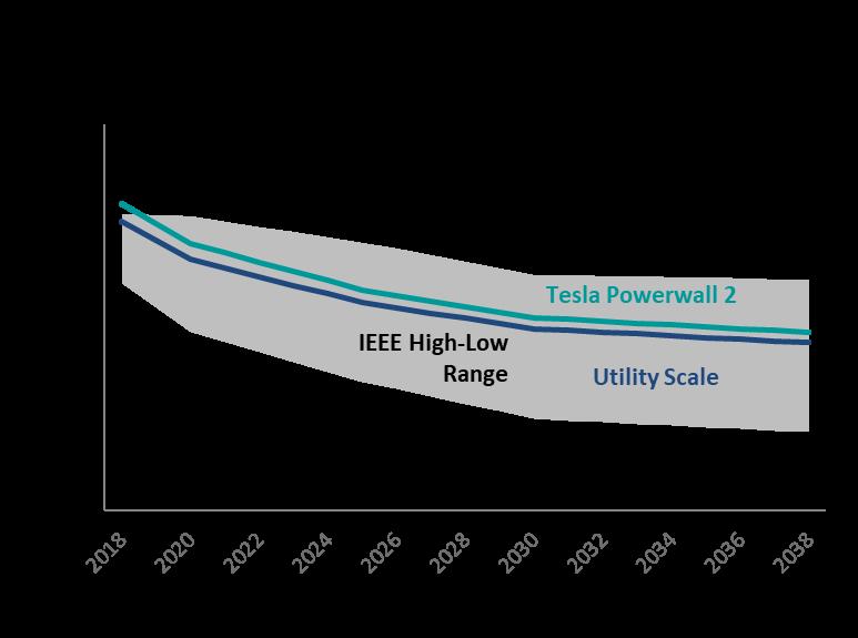
Further information about resource options and assumptions can be found in Chapter 5 and in Appendix A: Generating Resources.
Using assumptions for payback, considering assumptions unique to each scenario and strategy combination, the DG model provides forecasts for the following:
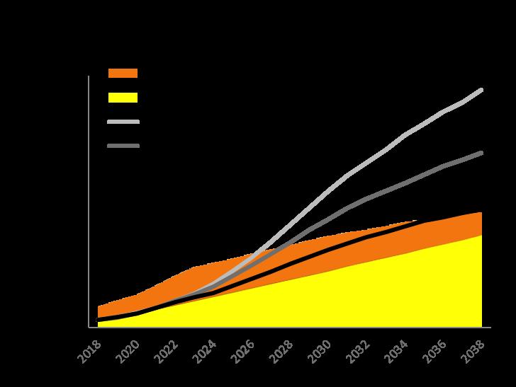
• Base levels of DG, considering TVA programs and payback without additional incentives
• Level of DG with moderate incentives
• Level of DG with high incentives
An example of the DG model output, specifically the resulting levels of DG adoption for Scenario 1 (Current Outlook), is shown in the figures below.

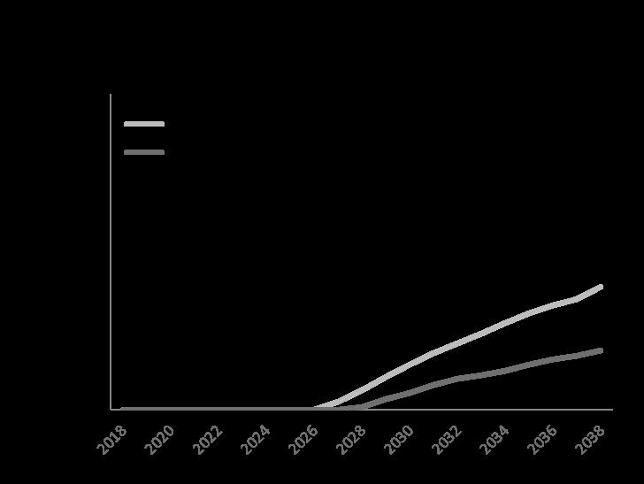
Once the DG profiles are created for distributed solar, distributed storage and CHP, they are imported into the expansion model. A unique set of DG adoption levels is fed into the expansion model for each scenario and strategy combination. The DG adoption levels are treated as required resources, or effectively a constraint the model has to operate with prior to optimization of other resources.
After the DG profiles for distributed solar, distributed storage and CHP are imported into the expansion model as required resources, the expansion model will then be run to optimize the remainder of the portfolio. This action is performed for each scenario and strategy combination, considering the aims and bounds of the strategy and all available generation and programmatic resources. The Reserve Margin is an important consideration in this step, ensuring that the expansion path chosen results in a portfolio that meets or exceeds seasonal reserve margin requirements to support a reliable system at the lowest feasible cost for a given strategy.
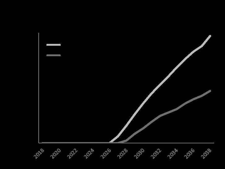
TVA’s 2019 IRP utilizes an innovative methodology to forecast the impact of different strategies on DG penetration across various future scenarios. The method simulated the effect of monetary incentives reducing payback and driving higher adoption of DG technologies. Results from the model allow TVA to gain insights into the impact that distributed generation could have on the TVA system under a variety of different future states. This knowledge will further inform future planning to meet TVA’s mission of providing reliable, low-cost energy to the residents of the Tennessee Valley.
In 2018, TVA conducted three studies to inform resource planning for an evolving system These studies focused on reserve margin, intermittent resources, and system flexibility. TVA’s system is essentially dual-peaking in the summer and winter, with a slightly higher forecast for the winter peak under normal weather conditions. With declining solar prices and increasing consumer demand for renewables, TVA anticipates thousands of additional solar megawatts will be added to the system over the next decade. Solar will not contribute to supply at the winter peak that typically happens early in the morning Also, there may be benefit to adding highly flexible resources such as battery storage or aeroindustry based combustion turbines (aero-derivatives) to support successful integration of additional renewables. The FY 2018 Resource Strategy Studies support planning for a future system that is low-cost, reliable, diverse, flexible and cleaner by:
• Updating reserve margins to support reliability in summer and winter peak seasons with more renewables expected on the system
• Recognizing sub-hourly costs driven by integrating intermittent resources onto the system
• Recognizing sub-hourly benefits driven by integrating highly flexible resources onto the system
These three studies utilized the same dataset based on TVA’s FY 2018 Budget Power Supply Plan. The reserve margin study was modeled at an hourly level The intermittent resources and flexibility studies were modeled at a sub-hourly level to understand the impact of solar and wind variability at that granularity, as well as the ability of highly flexible resources to respond to sub-hourly fluctuations. TVA’s capacity planning tool is an hourly model which considers operating characteristics of power resources at an hourly granularity. The relative flexibility (or inflexibility) of conventional resources such as
nuclear, coal and gas units can be seen at an hourly level Intermittent resources have hourly shapes but also have sub-hourly variability that cannot be seen in an hourly model. Likewise, highly flexible resources such as aero-derivatives and batteries provide subhourly flexibility, which cannot be seen in an hourly model. To fully capture characteristics of intermittent and highly flexible resources, additional study was needed. The studies will be used for both the 2019 IRP and annual capacity planning and will be repeated every few years or as changes in drivers warrant.
TVA used a third-party consultant, Astrapé Consulting, to run the Strategic Energy and Risk Valuation Model (SERVM), a state-of-the-art reliability and production cost simulation tool that employs a probabilistic view of costs and risks. SERVM was originally designed as a hybrid resource adequacy and production cost model by the Southern Company in the mid 1980s. Since then, the SERVM model has been used to identify planning and resource adequacy requirements, estimate the contribution of resources to reliability and flexibility requirements, as well as estimate the amount and operating characteristics of new resources to meet need. Astrapé Consulting provides resource adequacy studies for a number of large utilities nationwide. The implementation of SERVM for the FY 2018 Resource Strategy Studies included chronological simulations for the full 8,760 hours in a year with the following major inputs specific to the TVA system common across all three studies:
• Load: 30+ years of load shapes were developed using historical weather and current or projected weather/load relationships.
• Demand-side Resources: Program definitions with capacities, contractual constraints and dispatch rules were defined in the model. Typical constraints for demand response include hours per day, week, month, season and year, as well as call duration.
• Supply-side Resources: Supply side resources include nuclear, coal, combined cycle, combustion turbine, hydro, pumped storage and renewable resources within TVA’s portfolio, as well as the opportunity to
purchase power from neighboring regions. Variable operating costs related to fuel, startup, reagents, and operating and maintenance were modeled.
• Hydro Availability: Hydro resources were modeled to capture weather variations, operating range flexibility and ancillary service contribution. Input variables include monthly capacity and energy, as well as minimum and maximum flows on an hourly, daily, weekly and monthly basis.
• Ancillary Service Requirements: Regulation up, regulation down, spinning reserve requirements and targets, and non-spinning reserve requirements were defined by hour of day, month or year and as a function of load.
• Operating Reserve Requirements: TVA target operating reserve requirements of 3,050 MW include the following: 200 MW of regulating reserves at a five-minute response time, 1,350 MW of contingency reserves at a 15-minute response time, and 1,500 MW of replacement reserves at a 90-minute response time.
• Transmission: Import and export constraints for firm purchased power from neighboring regions were modeled for approximately 20 zones.
The following sections further explain the purpose, background, scope and approach, inputs, results, and conclusions stemming from each of the three studies.
Every few years, TVA performs a Reserve Margin Study to determine appropriate reserve margin planning targets to ensure resource adequacy for serving electricity demand in the Valley. The 2018 study focused on determining reserve margins for both summer and winter, accounting for seasonal differences in demand and supply.
TVA has a dual-peaking system, with additional thermal and hydro capacity in the winter but also greater weather-driven peak variability in that season. Meanwhile, declining prices and increasing consumer
demand is driving increased solar capacity in the future A study that considered seasonal differences in demand and in unit capabilities and performance, along with the potential for increased solar on the system, was needed to determine appropriate reserve margin planning targets for both summer and winter.
For the past several years, TVA used a 15 percent summer reserve margin target and a 20 percent winter reserve margin guideline, which translates to planning for at least 15 percent excess capacity over expected peak summer demand and at least 20 percent excess capacity over expected peak winter demand. Because prior studies for TVA focused on an annual reserve margin based on summer, this study was needed to inform targets for both peak seasons. Some regional peers are also exploring potential for using seasonal reserve margin targets. Every utility’s reserve margin equation is unique given each system’s supply and demand
Astrapé ran SERVM to capture the uncertainty that arises from unplanned events due to weather, load forecast error, and plant outages which drive the need for a planning reserve margin. To account for the variability of temperature, economic cycles, and plant outages, the study utilized 37 years of weather data under recent usage intensities, seven load forecast error points and 100 unit outage draws. The study also considered the load diversity of neighboring utilities and the ability to purchase firm power from those utilities. Overall, this resulted in more than 25,000 8,760-hour simulations that provided a robust view of what the TVA system could experience five years into the future. The five-year look-ahead allows time to build or acquire a resource or power purchase agreement, if needed.
The objective function of the study was to determine reserve margin targets that support an industry best practice level of reliability in both summer and winter, considering the expectation of more solar on the system. Industry best practice level of reliability is typically expressed as one loss of load event (LOLE) every 10 years, or 0.1 LOLE for one year. Seasonal reserve margins were determined through two approaches: 1) a physical reliability evaluation to achieve an annual target of 0.1 LOLE, and 2) an
The physical study was done in two ways, using a traditional approach adding back combustion turbines (CTs) and a revised approach adding back a
combination of CTs and solar to reflect the expectation of solar growth in the Valley.
The study approaches are further described in Table D-1.
CT Approach: Modeled reduced capacity and then added CTs until seasonal risk balanced to achieve 0.1 LOLE annually, or about 0.05 in each peak season.
CT & Solar Approach: Modeled reduced capacity and then added CTs to achieve 0.05 LOLE in the winter and solar to achieve 0.05 LOLE in the summer, resulting in balanced seasonal risk and an annual 0.1 LOLE
In addition to the common inputs mentioned in the Study Overview, the following inputs were included:
• Capacity reductions to model low reserve margin position (higher cost gas and coal units)
• 7 Load Forecast Error Points
• 100 Unit Outage Draws
• Incremental CT capacity (for CT Approach)
• Incremental CT and solar capacity (for CT & Solar Approach)
• Astrapé Consulting modeled neighboring utility systems, with excess capacity in the
Performed an economic evaluation to determine the reserve margin target that results in lowest cost to customers at a 90 percent confidence level.
region available to support replacement reserves
The study evaluated weather-driven variability around summer and winter peak loads, as shown in Figure
D-1. While summer peak loads have varied up to 8 percent around weather-normal conditions, winter peak loads have varied up to 15 to 20 percent around weather-normal conditions. Results indicated that winter peak load variability due to weather is more unpredictable and that additional reserve margin is required to ensure reliability in winter.
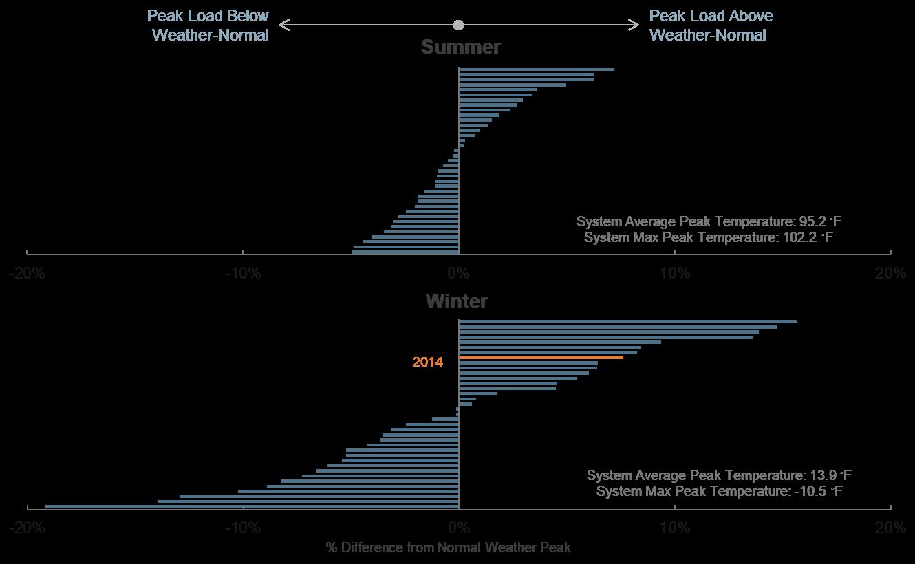
Also, there are notable differences in seasonal capacity. As shown below in Figure D-2, all resource types except for solar have higher winter capacity. Thermal units operate more efficiently in cooler temperatures, and more hydro generation is typically available in the winter. Solar resources contribute to
the summer peak, but do not contribute to the winter peak that typically happens around 7 a.m With the expectation of increasing solar on the system, there may be less difference in overall system winter and summer capacities in the future
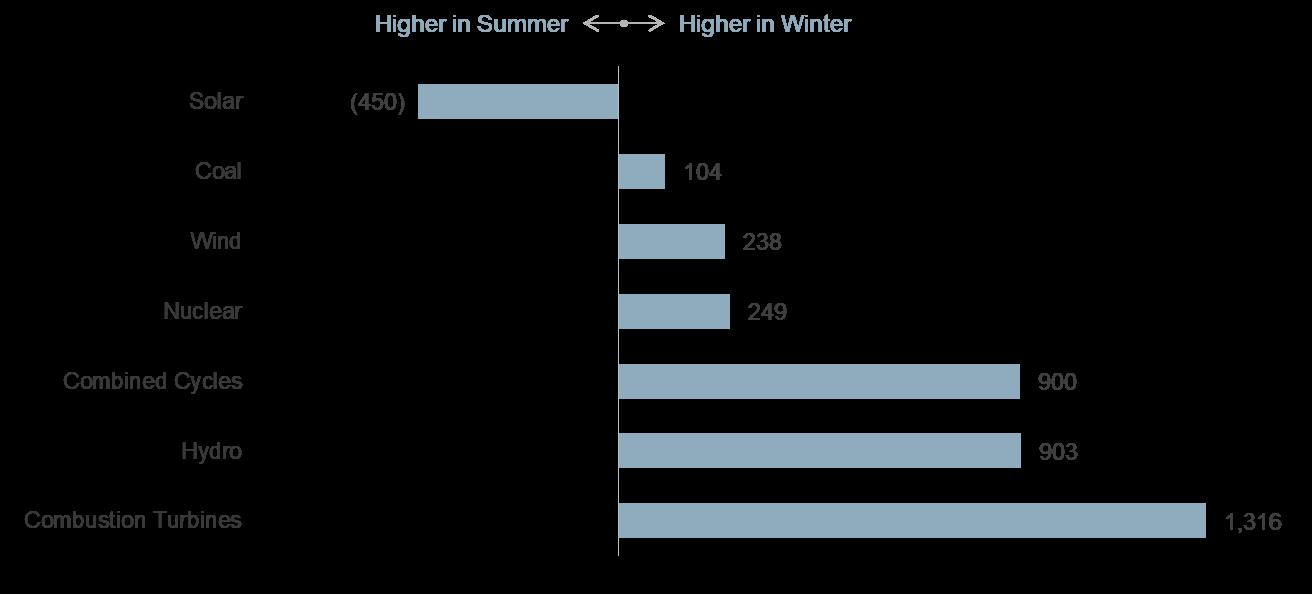
The physical reliability study indicates that TVA’s previously held summer and winter reserve margins of 15 percent and 20 percent equate to one loss-ofload event every four years, or 0.25 LOLE compared to an industry best-practice level of 0.1 LOLE. Anticipating more solar on the system over the next decade, the CT & Solar approach was adopted. Results from the study are summarized below in Figure D-3. The curve shows the various
combinations of summer and winter reserve margins that result in 0.1 LOLE, with about 2,500 MW of solar added in the simulation. Results indicate that a 17 percent summer reserve margin and a 25 percent winter reserve margin will achieve 0.1 LOLE and balance seasonal risk. The 2018 reserve margin position was approximately 20 percent in the summer and 30 percent in the winter. While the new reserve margin targets do not have an immediate impact, they will inform future resource decisions.
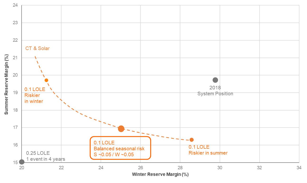
The economic evaluation measured four cost components across various reserve margin levels in the study results to identify the reserve margin that would yield the minimum cost at a 90 percent confidence level. The four cost components are:
• Incremental Production Costs: Represents costs such as variable fuel, operations and maintenance costs that are incurred by conventional assets.
• Renewables: Represents costs associated with adding solar resources. As solar is
added, incremental production costs decrease while renewable costs increase.
• Net Purchases: Represents the net cost of purchasing and selling energy from outside TVA’s system. More generating capacity within the system reduces the need to purchase.
• Expected Unserved Energy: Represents the costs associated with an interruption in service, estimated at $15,000/MWh based on a London School of Economics study used by many utilities. The greater the reserve margin, the less likely an interruption is to occur.
Results from the economic evaluation (Figure D-4) indicate that the minimum cost occurs at a summer reserve margin of 16.75 percent, with negligible
difference in cost (less than $1 million) between that level and the 17 percent target derived from the physical reliability approach.
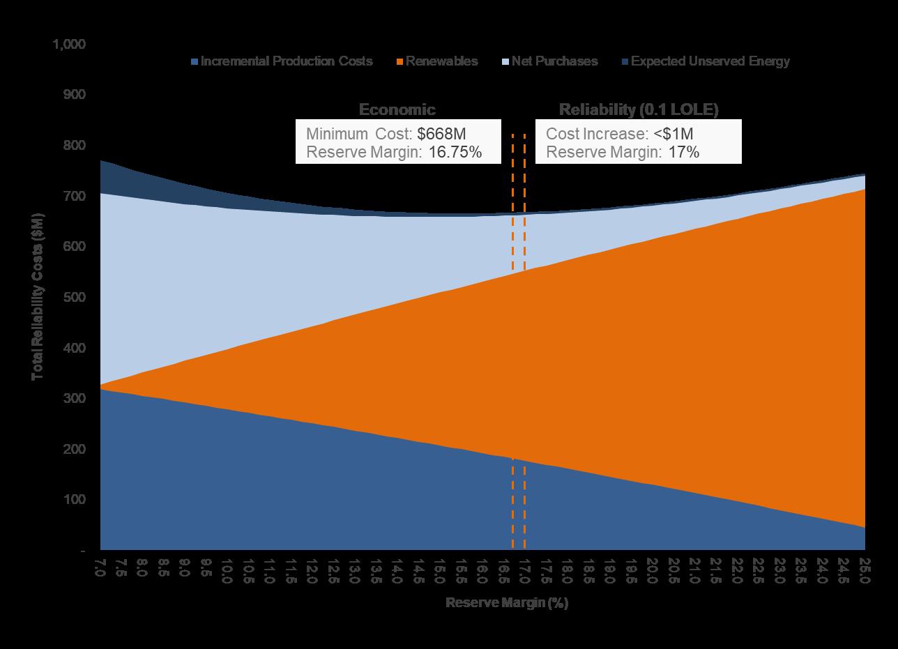
TVA’s targets are in alignment with its neighbors, given differences in load and supply, shown in Figure D-5. While many systems only have one target
reserve margin, according to NERC’s 2018 LongTerm Reliability Assessment and other systems’ IRPs, there is a growing trend in having seasonal separation in reserve margins
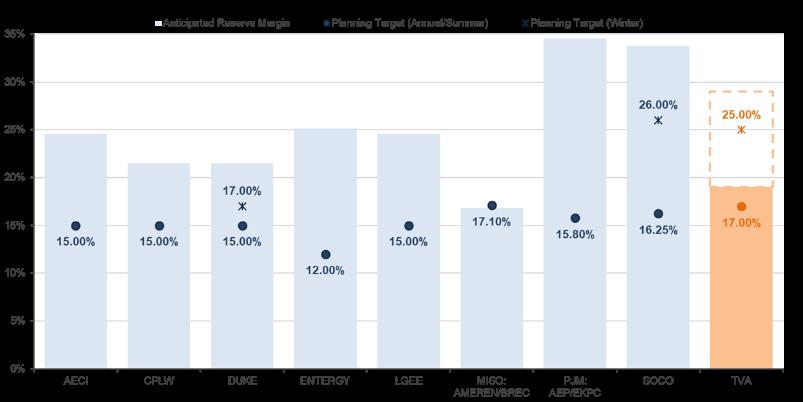
Based on study results, TVA planning reserve margin targets of 17 percent in summer and 25 percent in winter were recommended for use in resource planning to align with industry best-practice LOLE of one event in 10 years, balance seasonal risk and achieve minimum cost.
Updated seasonal reserve margin targets better position TVA to ensure resource adequacy for our dual-peaking system with expectations for increased solar in the Valley. The summer and winter reserve margins are being used in the 2019 IRP as well as in annual resource planning. TVA expects to update the Reserve Margin Study before the next IRP or as changes in drivers warrant.
The purpose of the Intermittent Resources Study was to improve TVA’s understanding of reliability and economic impacts to the portfolio as intermittent resource penetration increases. With declining solar costs and increasing consumer demand for renewables, TVA expects to see more solar on the system in the next decade Whether solar is in front of or behind the wholesale meter, TVA’s system will need to absorb intermittency impacts and maintain reliability. Specifically, the study sought to identify the
net dependable capacity of solar and wind resources and the sub-hourly impacts of these resources at various penetration levels. The results from the study can be applied in hourly capacity planning models to more fully reflect the impacts of adding intermittent resources on the system.
As solar and wind generation is intermittent and has unique shapes, it is important to understand the dependability of this generation at TVA’s summer and winter peaks. The seasonal capacity of intermittent resources can be represented by Net Dependable Capacity (NDC) or Effective Load Carrying Capacity (ELCC). NDC calculates a 75 percent confidence of capacity at the peak hour of the top 20 days of highest load. ELCC determines the equivalent capacity of wind or solar compared to a dispatchable plant’s ability to avoid a loss of load event. This study evaluated both methods to determine the appropriate capacity for use in resource planning.
The intermittency of solar and wind generation presents some operational challenges, such as requiring other generating units to provide additional load following and cycling to absorb sub-hourly fluctuations. The cost of these challenges is referred
to as an integration cost For the past several years, TVA used a proxy for integration costs based on other utility studies, specifically $5/MWh for solar and $8/MWh for wind. A detailed study of TVA’s system was needed to determine the additional cost of maintaining system reliability as more resource intermittency is introduced.
Integration costs were defined by the two components, additional operating costs and maintenance costs, explained further as follows 1:
• Operating Costs: Costs incurred from additional load following, curtailments, and cycling of gas, coal, and hydro resources to maintain generation-load balance with subhourly fluctuations in intermittent resources.
• Maintenance Costs: Costs incurred for maintenance on boilers, turbines, generators and switchyards from the additional cycling of resources that help maintain generation-load balance.
To determine the impacts of introducing additional intermittent resources to the portfolio at various penetration levels, this study sought to:
• Define the seasonal capacity of intermittent resources by selecting either the Net Dependable Capacity (NDC) or Effective Load Carrying Capacity (ELCC) method
• Identify the sub-hourly integration cost for varying levels of intermittent resource penetration for use in hourly resource planning models.
The first step was to evaluate NDC and ELCC methods to determine the best approach for intermittent resource seasonal capacity. Since the NDC method is based on historical trends, TVA analyzed the capacity factor for each solar and wind contract for 30 historical years. In contrast, the ELCC method measures renewable capacity by replacing peaking capacity. Through a reliability model, solar or
wind capacity is added to a reference case and peaking capacity is removed until the LOLE is equal to the reference case. ELCC is derived using the ratio of the renewable capacity to the peaking capacity.
The second step was to evaluate sub-hourly integration costs for solar and wind resources. This study sought to develop an integration cost curve specific to TVA’s fleet that would represent the cost of maintaining system reliability as more intermittency is introduced to the portfolio. As intermittent resource penetration increases, it is expected that integration costs will increase. The objective was to determine the appropriate sub-hourly cost to use in resource planning given expected level of renewable penetration over the next decade, so that early and late additions would share equal burden This approach is similar in concept to all houses in a new development sharing the cost of a sub-station transformer upgrade, rather than only the last few houses built bearing that cost.
To model integration costs, solar and wind resources were modeled at five-minute granularity to more fully capture intermittency patterns, and then these resources were added to the portfolio at various penetration levels (Figure D-6). The model was run at both an hourly and sub-hourly level, and then results from the sub-hourly run were subtracted from the hourly run to isolate the sub-hourly impacts of intermittency with no overlap with hourly energy benefits and impacts. The results from the run comparisons inform the integration cost curves.
In addition to the common inputs mentioned in the Study Overview, the following inputs were included:
• Incremental solar capacity at 2,500 MW, 5,500 MW, and 9,500 MW penetration levels
• Wind capacity at 3,000 MW penetration level
1 Integration cost components may also include flexible reserve costs, which include the carrying cost of additional flexible
D.3.5.1 Net Dependable Capacity resources, and transmission costs, which include the cost of additional transmission system capability. These components were also analyzed in this study, but no costs were specifically identified
After evaluating both the NDC and ELCC methods to determine solar and wind capacity, study results indicate that a mixed approach is most suitable.
Peak capacity contribution of wind varies greatly from year to year. Thus, NDC is the preferred method because it considers every year of historical performance to determine capacity contribution, whereas ELCC only looks at the years of loss-of-load expectation due to high load or low plant availability.
Using the NDC approach, wind capacity at peak would be valued at 14 percent in summer and 31 percent in winter This result is similar to the results from a 2016 MISO study that evaluated dependable capacity of wind from a similar geographic region at a similar level of penetration.
As solar generation at the summer and winter peaks tends to be fairly consistent year to year, ELCC is the
preferred method for solar peak capacity contribution. Using the ELCC approach, solar capacity at peak would be valued at 68 percent in summer and 0 percent in winter. The study found contribution to winter peak, typically around 7 a.m., to be less than 1 percent. Increasing solar penetration typically shifts the summer peak and reduces ELCC, as has occurred in regions with higher solar penetration, and future ELCC studies will be able to capture this impact.
Study results for solar and wind integration costs at additional penetration levels are summarized in Figure D-6 The results also show the breakdown between additional operating and maintenance costs.
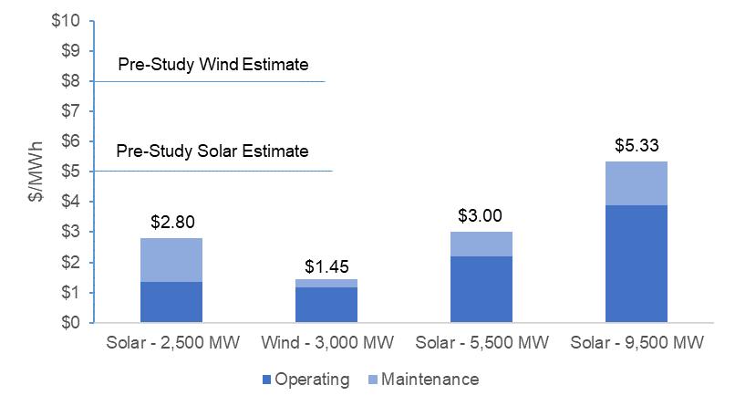
Results overall were notably lower than pre-study estimates. Projected solar integration costs averaged about $3/MWh from 2,500 MW to 5,500 MW penetration, then began increasing up to about $5.5/MWh at 9,500 MW penetration. Projected wind integration costs were about $1.5/MWh at 3,000 MW additional penetration. With the diversity of the portfolio, including the ability to leverage the flexibility of conventional hydro assets, the TVA system is well
positioned to absorb up to 5,500 MW of solar and 3,000 MW of wind at relatively small additional cost
Other utilities and Independent System Operators have conducted studies to evaluate the challenges and costs associated with integrating renewable resources. One of the most comprehensive studies was performed by Synapse in 2015 Synapse
researched integration costs and found that system operators implemented measures to integrate large amounts of wind and solar resources at costs generally less than $5/MWh of energy produced At the time of this publication, more information about the Synapse study was available on the Synapse website at the following link:
http://www.synapse-energy.com/sites/default/files/Costsof-Integrating-Renewables.pdf
Integration costs are only a piece of the equation, and other factors such as state renewable mandates or goals, declining solar prices, regional capacity factors, cost of competing resources, and consumer demand are playing into resource selection and timing. Understanding the impacts of intermittency also informs the need for flexible resources to support successful integration of renewables.
Based on study results, summer and winter net dependable capacities of 68 percent and 0 percent for solar and 14 percent and 31 percent for wind will be used. Given TVA’s system is well-positioned to absorb up to 5,500 MW of solar and 3,000 MW of wind and current projections are within those bounds for the next decade, study results from those penetration levels informed the recommendation Sub-hourly integration cost results were rounded to $3/MWh for solar and $2/MWh for wind for use as inputs in resource planning. These planning factors account for the contribution of solar and wind at TVA’s summer and winter peaks and for the subhourly costs of intermittency that can be captured in TVA’s hourly resource planning models
Identifying net dependable capacities and sub-hourly integration costs for solar and wind resources provides a fuller picture of the operating characteristics of intermittent resources to inform resource selection. The following section further explores the relationship between increasing penetration of intermittent resources and the value of more flexible resources on TVA’s system. The NDCs and integration costs are being used in the 2019 IRP as well as in annual resource planning. TVA expects to update the Intermittent Resources Study before the next IRP or as changes in drivers (including intermittent resource penetration) warrant.
The purpose of the Flexibility Study was to understand the potential benefits of adding more flexible resources on the system and how those benefits may change as renewable penetration increases. The study sought to identify the sub-hourly impacts of introducing highly flexible resources to the portfolio at various levels of intermittent resource penetration. Study results can be applied in hourly capacity planning models to more fully reflect the impacts of adding more flexible resources to the portfolio.
The Intermittent Resources Study and Flexibility Study go hand in hand, in that they reflect two sides of the same equation. While intermittent resources introduce additional sub-hourly variability in operations, highly flexible resources introduce additional sub-hourly flexibility in operations. Over the next decade, TVA expects to see more solar on the system, both behind and in front of the wholesale meter. It is important to understand the full value that highly flexible resources can offer now and in the future so that value can be proactively considered in capacity planning.
This study evaluated the benefit of highly flexible resources, specifically aero-derivative combustion turbines and lithium-ion batteries, with increased solar generation in TVA’s system. Specifically, this study sought to:
• Identify sub-hourly flexibility benefits of adding aero-derivatives, batteries, hydro and pumped storage to the portfolio at varying levels of penetration
• Determine how this benefit changes at differing solar penetration levels.
This first step involved determining a set of operating parameters for aero-derivatives, batteries, hydro and pumped storage. Figure D-7 highlights study assumptions about aero-derivatives relative to frame combustion turbines (CTs), currently the most flexible resource in TVA’s portfolio. Compared to frame CTs,
aero-derivatives have more efficient heat rates, quicker ramping capability, and no start costs, which make them attractive from a flexibility perspective.
in their ability to efficiently store energy for use at other times
The second step involved evaluating the sub-hourly flexibility benefits of existing hydro and pumped storage and potential aero-derivative and battery capacity. The objective was to determine the appropriate benefit to use in resource planning given expected level of renewable and flexible resource penetration over the next decade. To model flexibility benefits, SERVM was populated with TVA’s load forecast and current portfolio of assets.
To analyze the benefit of the two existing technology types, hydro and pumped storage, their capacities were initially removed. About 2,500 MW of solar generation was added at five-minute granularity, aligning to base case penetration expectations evaluated in the Reserve Margin Study. Then, flexible capacity was added at various levels of penetration. Hydro capacity was modeled by mimicking historical sub-hourly profiles with +/-100 MW of operating flexibility within each hour. For pumped storage, each of TVA’s four 424 MW pumped storage units was added incrementally. Capacity was modeled such that all units were in generating or pumping mode with one hour idle time required between changes in directional operation. A comparison of hourly and sub-hourly runs was used to identify the flexibility value of the existing hydro and pumped storage fleet.
For the two potential technology types, aeroderivatives and batteries, increasing amounts of capacity was added to evaluate the impacts on overall system operations and cost. Similar to the
Intermittent Resources Study, the model was run at both an hourly and sub-hourly level. Then, results from the sub-hourly run were subtracted from the hourly run to isolate the sub-hourly impacts of flexibility with no overlap with hourly energy benefits and impacts. The analysis was also run at 5,500 MW of solar penetration to evaluate the relationship of increased intermittency and flexibility value. The results of the study inform the flexibility benefit curves at various flexible resource and intermittent resource penetration levels.
In addition to the common inputs mentioned in the Study Overview, the following inputs were included:
• Aero-derivative Capacity (200 MW, 500 MW, and 1,000 MW) with study parameters
• Battery Capacity (200 MW, 500 MW, and 1,000 MW) with study parameters
• Conventional Hydro Capacity (3,000 MW) with study parameters
• Pumped Storage Capacity (1,696 MW added unit by unit) with study parameters
• Solar Capacity (2,500 MW, and 5,500 MW)
The ability to leverage the flexibility of the current hydro and pumped storage fleet contributes benefits of $23/kW-year and $2.9/kW-year, respectively Hydro provides flexibility every hour throughout the
year, and could provide additional savings if the operating range could be expanded. Simulations showed that, while pumped storage has a great deal of energy benefit hour to hour, its operating characteristics limit sub-hourly flexibility value.
At solar levels consistent with the Reserve Margin Study, the Flexibility Study indicated decreasing benefits with increasing penetration of new, highly flexible resources. Results show that adding 1,000 MW of aero-derivatives or batteries would drive benefits of about $9.5/kW-year and $1.7/kW-year, respectively. Simulations showed that aeroderivatives averaged two starts per day and an annual capacity factor of 23 percent, and that aeroderivative benefits may be higher in peak months and
battery benefits may be higher in shoulder months. Flexibility values were derived by taking the net present value of the benefits achieved when operating the system more efficiently with the addition of more flexible resources. Solar integration costs of $3/MWh can also be expressed as $6.5/kW-year, as a relative comparison for these results.
Additionally, model results indicated that the flexibility benefit for aero-derivatives and batteries increased at higher levels of solar penetration. The flexibility value increased by a higher percentage for batteries than for aero-derivatives. Figure D-10 below summarizes the flexibility benefits of varying levels of aeroderivatives and batteries at two different solar penetration levels.
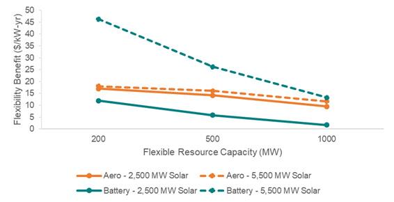
Based on study results, sub-hourly flexibility values of $9.5/kW-year for aero-derivatives, $1.7/kW-year for batteries, $23/kW-year for hydro, and $2.9/kW-year for pumped storage were recommended for use in resource planning. Hydro and pumped storage values would be applied on a pro-rata basis to expansion options that impact overall hydro system operating range or pumped storage capability. These planning factors account for the sub-hourly benefits of highly flexible resources that can be captured in TVA’s hourly resource planning models
Including a sub-hourly benefit for highly flexible resources provides a fuller picture of the operating characteristics of highly flexible resources to inform resource selection. This benefit would be expected to increase with increasing intermittent resources on the system. The flexibility benefit is being used in the 2019 IRP as well as in annual resource planning. TVA expects to update the Flexibility Study before the next IRP or as changes in drivers (including penetration of new flexible resources) warrant.
This page intentionally left blank.
With robust input from the IRP Working Group, TVA developed five different future environments that,
coupled with the TVA’s Current Outlook, constitute the six scenarios described in Figure E-1.
•Economic outlook reflects slowing expected in 2020, transitioning to a long-term growth rate of 2 percent for TVA region GDP and 1.9 percent inflation
•Demographic changes slow customer count growth, while declining household size and increasing efficiencies drive lower energy use per customer
•Gas supply more than adequate to meet demand, and power prices follow seasonality of gas prices and volatility of weather
•Prolonged, stagnant economy results in weak growth and delayed expansion of new generation
•Ballooning budget deficits and public debt hit record levels constraining federal economic policy actions
•More tariffs on U.S. imports are followed by retaliatory tariffs on U.S. exports
•Stringent environmental regulations delayed due to concerns of adding further pressure to economy
•Weaker demand lowers cost of new plant construction
Decarbonization
•Technology-driven investment in automation and artificial intelligence raise electricity use, boosting labor productivity and economic growth while lowering inflation
•Rapid economic growth, driven by migration into the Valley and growth in emerging markets and developing economies, translates into higher energy sales
•Lower battery costs due to economies of scale drive electrification of transportation, magnifying growth
•Preference for lower emissions, DER, and EE lowers demand for emitting generation, translating into lower gas and coal prices
•Increasing climate-driven effects create strong federal push to curb greenhouse gas emissions, increasing CO2 emission penalties for the utility industry and incentives for non-emitting technologies
•Compliance with new rules increases energy prices and US-based industry becomes less competitive, resulting in lagging economic growth that fails to rebound to trend levels
•Fracking regulations never materialize, but gas demand is impacted by CO2 penalty
•New gas expansion units are necessary to replace existing higher CO2-emitting fleet
No Nuclear Extensions
•Growing consumer awareness of and preference for energy choice, coupled with rapid advances in energy technologies, drive high penetration of distributed generation, storage & energy management
•Utilities are no longer the sole source of generation and multiple options are available to consumers
•Market shift results in lower loads, decreased need for supply-side generation, but potential impacts to transmission and distribution planning and infrastructure
•Driven by aging assets and desire for national energy security and resiliency, there is a regulatory challenge to relicensing of existing, and contruction of new, large scale nuclear plants.
•National energy policy drives carbon regulation or legislation and promotes small modular reactor (SMR) technology through subsidies to drive advancements and improved economics
An overarching principle in the design of scenarios was to ensure a wide range of possible outcomes. To
that end, the uncertainties that impact possible futures were altered in such a manner as to cause a range of
impacts from none to very low to very high, as shown in Figure E-2
In each scenario, uncertainties were levered to reach the desired end-state For example, in the Valley Load Growth scenario, a very high penetration rate of electric vehicles was used to reach “very high” outcomes for Electricity Demand and Electrification.
One of the major challenges to translating the uncertainties into model results is defining what is meant by the categories ranging from “very high” to “very low,” ascribing numbers to those definitions and then actually achieving the desired results. The uncertainties that affect electricity usage the most, and that are the focus of this section, are Economic
Outlook, Electrification, and Distributed Generation Penetration, which are, in turn, affected by solar, storage and natural gas prices, and regulations.
Two of the scenarios were directly affected by economics - the Economic Downturn and Valley Load Growth scenarios A third scenario, Decarbonization, saw economic impacts as a result of regulations and had a regional GDP growth rate midway between the Current Outlook and the Economic Downturn (See Figure E-3) The No Nuclear Extensions and Rapid DER Expansion cases both aligned with the Current Outlook trajectory In all scenarios, the economic assumptions were applied for the full twenty years of the study period (2019-2038) In the Economic Downturn scenario, for example, normal business cycle effects were removed and low economic growth
occurred in each of the twenty years The same logic holds for the Valley Load Growth and
Decarbonization cases This approach was taken to help drive greater breadth of results.


+14% -7% -15%
The economic drivers mainly impact electricity demand by increasing or decreasing business or consumer investment. With anemic economic growth, weaker demand results in lower capital investment in manufacturing plants by businesses or distributed generation by individuals. In a growing economy, the opposite is true with larger investments in electrification, energy efficiency, business expansion and distributed generation.
The ability to invest was a significant driver to the large penetration of electric vehicles (EVs) in the Valley Load Growth scenario In that case, every new vehicle sold by 2038 light, medium and heavy duty along with transportation (buses) will be electric, translating into almost five million EVs on the road in the Valley Energy-wise, the lowest penetration occurred in the Current Outlook and No Nuclear Extensions cases because they only included light duty vehicles, which are less energy intensive The
Economic Downturn case had less than 500,000 EVs (see Figure E-4), but more energy usage because it had a mix of light, medium, heavy duty and buses. For the other two cases, the drivers to growth are dictated more by preference or regulation as outlined in the scenario narratives. Electric vehicles are the only representation of electrification in the residential sector.
Investment was also an important driver for business electrification and expansion as shown in Figure E-5 Large Commercial and Industrial (C&I) customers added the most electricity usage in the Valley Load Growth scenario with a very high 1.9 percent compound annual growth rate (CAGR) over the twenty years from 2018 to 2038. In that case, businesses expanded as a result of economic growth inside and outside the Valley The Valley population grew faster than the nation as a whole because of inmigration to the TVA service territory from other parts
of the country Also, large data centers came online in the Valley, adding even more electricity growth The Current Outlook, Decarbonization, Rapid DER Expansion and No Nuclear Extensions cases showed modest Large C&I growth of 0.3 percent per year.
The Economic Downturn case showed Large C&I decline of 0.7 percent per year as businesses struggled Residential customers also struggled and were more conscious of energy bills, driving additional energy conservation.
Distributed Generation penetration, represented by solar, battery storage and combined heat and power (CHP), was not only impacted by ability to invest but also by regulation, customer preference and natural gas prices. Renewable generation, attributed to only behind-the-meter (BTM) solar with batteries, was equal to or higher than the Current Outlook in every case (Figure E-6). The anticipated lower future prices of installed solar along with various incentives drove much of the increases Batteries, reliant on excess solar generation to charge, were present in many of the cases as noted within the table in Figure E-6. The Rapid DER Expansion scenario had the highest impact from BTM solar by far because technology breakthroughs greatly decreased the cost. The penetration occurred both in the residential and Large C&I sectors, with some customers able to go off-grid and use TVA only for back-up power needs. The Decarbonization case had the next highest impact with penetration driven mainly by federal incentives,
as well as lower cost Cost was less of an issue in the Valley Load Growth scenario, but lower incentives meant the economics were less favorable, leading to lower renewable growth Renewable growth for the Economic Downturn and No Nuclear Expansions cases was the same as for the Current Outlook.
Another aspect of distributed generation was combined heat and power (Figure E-7) The Current Outlook, as well as the Decarbonization and the No Nuclear Extensions cases, had eight MWs per year of CHP growth for the first ten years of the forecast and none thereafter The Economic Downturn cut that in half, but the Valley Load Growth Scenario doubled the Current Outlook case The largest impact occurred in the Rapid DER Adoption scenario, where an average of 90 MWs of CHP was installed per year for the 20-year period. The drivers to this significant increase were lower technology cost along with the lowest natural gas prices of all scenarios evaluated.
The final uncertainty affecting the amount of electricity supplied by TVA was regulation through Department of Energy Codes and Standards for electrical appliances, motors, etc In Figure E-8, the impacts are shown as change in efficiency gains from the Current Outlook, represented as the zero line Not surprisingly, the Decarbonization case with its more stringent federal regulations was the scenario that
(10,000) (5,000)
(35,000) (30,000) (25,000) (20,000) (15,000)
(45,000) (40,000)
showed the largest impact Next came the Rapid DER Adoption, mainly driven by the lower cost of more efficient technology The Valley Load Growth scenario also had more efficiency since more investment dollars were available. Conversely, the Economic Downturn case had less efficiency as equipment turnover slowed due to weak economics.
To provide a view of the most impactful uncertainties or levers for each scenario, Figure E-9 shows the increase or decrease in gigawatt-hours of energy in 2038 for each scenario by driver, as compared to the Current Outlook. For the Economic Downturn scenario, Large C&I declines drove lower loads In the Valley Load Growth case, the proliferation of EVs
combined with data center and Large C&I growth caused load to grow faster than any other scenario. Regulations in the Decarbonization case drove higher levels of energy efficiency, mainly through DOE codes and standards. Penetration of solar and CHP behind the meter drove loads to their lowest levels overall in the Rapid DER Adoption case.
Varying these uncertainties across scenarios resulted in a wide range of future peak load and energy requirements to be served by TVA (Figure E-10).

Commodity prices include those for coal, natural gas, and carbon dioxide (CO2) Some of the scenario narratives addressed the expected direction of prices explicitly. Electricity demand, and consequently fuel demand, was lower in all scenarios but the Valley Load Growth and No Nuclear Extension scenarios
Lower demands generally result in lower prices especially with no externality to constrain supply
For natural gas (Figure E-11), the scenario narratives and uncertainty direction explain most of the movement The Economic Downturn scenario saw demand and price declines relative to the Current
Outlook. For the Valley Load Growth case, slightly higher demand coupled with the CO2 penalty in 2025 drove prices higher, especially after 2025 The Decarbonization case had the highest CO2 penalty and the highest gas prices with two, step increases: one in 2025 and the other in 2035, coinciding with the timing of the carbon penalty For the Rapid DER Expansion scenario, loss of electricity demand because of high penetration of BTM generation resulted in the lowest demand for natural gas and the lowest prices. The No Nuclear Extension case had the same price trajectory at the Current Outlook until 2033 when the generation loss from retiring nuclear plants caused additional generation from natural gas plants
While natural gas prices in the scenario range above and below the Current Outlook, coal prices in the long-term all fall at or below the Current Outlook (Figure E-12) The basic outlook for the coal markets was that no additional coal plants were to be constructed; hence, the aggressiveness of coal plant
retirements impacted demand along with the shift to other technologies In all cases, demand for coal was lower than the Current Outlook, which drove prices lower in all cases.
One externality addressed in this section is CO2.
Figure E-13 shows the price of CO2, expressed as dollars per ton emitted, for the scenarios Only the Valley Load Growth and Decarbonization cases had values different from the Current Outlook In the Valley Load Growth scenario, the robust economic situation provided the money to pay for the
preference for lower emissions that saw a CO2 penalty of $5 per ton beginning in 2025, escalating at inflation In the Decarbonization case, the stringent regulatory environment meant that a larger carbon penalty of $25 per ton commenced in 2025 That penalty escalated at the inflation rate, and in 2035, was ratcheted higher by another $10 per ton.
As depicted previously in Figure E-10, one of the key outcomes desired from the scenarios was a wide range of future energy profiles for TVA to understand. Figures E-14 and E-15 show a comparison of the annual peaks and annual energy, respectively, for the 2015 and 2019 IRPs. For the annual peaks and energy, the 2015 IRP had no scenario where the annual peaks and energy at the end of the study period was lower than the first year (2014) of the study In the 2019 IRP, half of the scenarios are lower in the twentieth year of the study as compared to the first year
By the last year of the study period, the annual peak distribution is twice as wide in the 2019 IRP as the 2015 IRP, with the Valley Load Growth case 39 percent higher than the Current Outlook and the Rapid DER Adoption scenario 13 percent lower. Also, by the last study year, the annual energy distribution is two and a half times as wide for the 2019 IRP compared to the 2015 IRP, with the Valley Load Growth scenario 48 percent higher and the Rapid DER Adoption case 26 percent lower than the Current Outlook.


Developing wide ranges of possible outcomes through the use of various uncertainties provides the means for creating electricity usage outcomes that stretch the boundaries of our thinking and planning.
With input from the IRP Working Group, TVA developed different business strategies to be applied across various futures to gain insights into potential
Strategies
Base Case
Promote DER
Promote Resiliency
Promote Efficient Load Shape
Promote Renewables
future resource portfolios. The combination of the six scenarios and five strategies being evaluated in the IRP will result in 30 unique resource portfolios
For each strategy, a narrative was developed to describe the promotion or constraint of certain resource types. These narratives, summarized in Figure F-2, provide a general roadmap for how the strategies should be designed
Description and Attributes
• Planning Reserve margins for summer and winter peak seasons are applied, targeting an industry best-practice level of reliability.
• No specific resource types are promoted beyond business as usual.
• DER is incented to achieve higher end of long-term penetration levels.
• New coal is excluded. All other technologies are available while EE, demand response, distributed generation and storage are promoted.
• Small, agile capacity is incented to maximize flexibility and promote ability to respond to short-term disruptions on the power system.
• All technologies are available while small modular reactors (SMRs) and gas additions (aero-derivative turbines, reciprocating engines), demand response, storage and distributed generation are promoted.
• Combinations of storage and distributed generation could be installed as microgrids.
• Flexible loads and DERs are aggregated to provide synthetic reserves to the grid to promote resiliency.
• Targeted electrification and demand and energy management are incented to minimize peaks and troughs and promote an efficient load shape.
• All technologies are available but those that minimize load swings, including EE, DR and storage, are promoted.
• Programs targeting low-income customers will be a part of EE promotion.
• Renewables at all scales are incented to meet growing prospective or existing customer demands for renewable energy.
• New coal is excluded. All other technologies are available while renewables are promoted.
Two different mechanisms for promoting a resource were considered: 1) targeting a higher penetration level for a promoted resource or 2) applying an economic incentive that effectively reduces cost for
the resource selection process. TVA opted to use an economic incentive approach, as a consistent incentive structure could be applied across the diverse set of resource options being promoted in the IRP. In practice, an economic incentive could be delivered in various ways, such as through a rebate, service, or pricing product. The incentive structure approach is shown in Figure F-3.
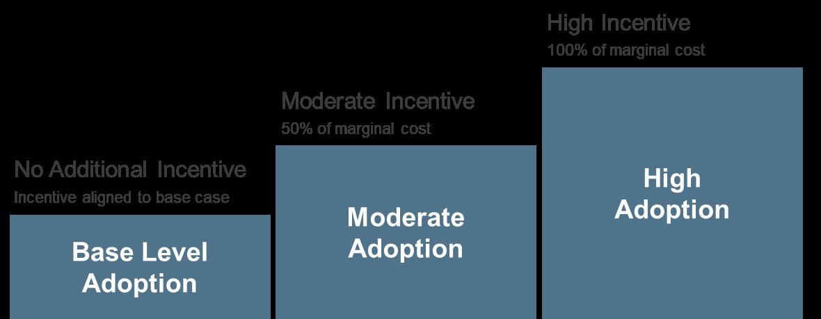
A base incentive level represents business as usual, or no additional incentive beyond continuation of existing programs. To promote adoption of a resource, a moderate or high incentive is applied. A moderate incentive is represented as 50 percent of marginal cost, and a high incentive is represented as 100 percent of marginal cost. For most resources, short-term marginal energy cost is used as the incentive, except for demand response, where shortterm marginal capacity cost is used. The ability of a particular resource to provide capacity is still considered in the optimization model, even though the incentive is generally based on marginal energy cost. Another exception is storage, which is promoted
based on the level of distributed or utility-scale solar incented in a portfolio at a 10 percent match for a moderate incentive and a 25 percent match for a high incentive. This incentive structure was applied across all promoted resources in the 30 unique scenario and strategy combinations.
A Strategy Design Matrix (Figure F-4) was developed to translate the narratives into a plan for promoting resources This matrix was used to guide the promotion of resources in the capacity planning model.
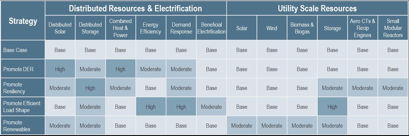
The Strategy Design Matrix includes resources promoted in one or more strategies across the top, along with a row for each strategy A number of factors were considered in final strategy design,
including IRP Working Group and Regional Energy Resource Council feedback, relative economics of promoted resources, alignment within a strategy, and differentiation across strategies
The Base Case strategy has no additional incentives beyond continuation of existing programs, so a “base” incentive level is listed for all resource types. Included in the Base Case is the continuation of the Low Income EE pilot program. Resources that are not promoted in the other strategies are also listed as “base” to indicate alignment to the Base Case All the strategies except the Base Case promote a unique set of resources, in most cases with a combination of moderate and high incentives.
The Promote DER strategy includes an incentive for all types of distributed energy resources and energy efficiency. Distributed solar and CHP receive high incentives in this strategy, and a moderate incentive is applied to distributed storage, energy efficiency, and demand response. Low Income EE is a subset of energy efficiency programs, and in this strategy, the pilot program is expanded Valley-wide.
The Promote Resiliency strategy includes an incentive for small, agile resources that support system flexibility to respond to dynamically changing loads and those that support local resiliency. Distributed storage receives a high incentive in this strategy A moderate incentive is applied to distributed solar, CHP, demand response, as well as to utility-scale storage, small gas assets (aeroderivatives and reciprocating engines), and small modular nuclear reactors.
The Promote Efficient Load Shape strategy includes incentives for resources that help shave peaks and fill valleys, making the overall system load shape more efficient. Utility-scale storage, along with energy efficiency and demand response, receive high incentives in this strategy A moderate incentive is applied to distributed storage and beneficial electrification. Low Income EE is a subset of energy efficiency programs, and in this strategy, the pilot program is expanded Valley-wide and incentives are increased.
The Promote Renewables strategy includes incentives for renewables at all scales, as well as for storage to support integration of renewables A moderate incentive is applied to distributed solar and storage, as well as to utility-scale solar, wind, biomass/biogas, and storage.
A number of strategies in the IRP explore promotion of distributed generation and storage. For the 2019 IRP, TVA developed an innovative way to model adoption of distributed generation (DG) technologies Figure F- 5 provides a high level summary of the methodology.
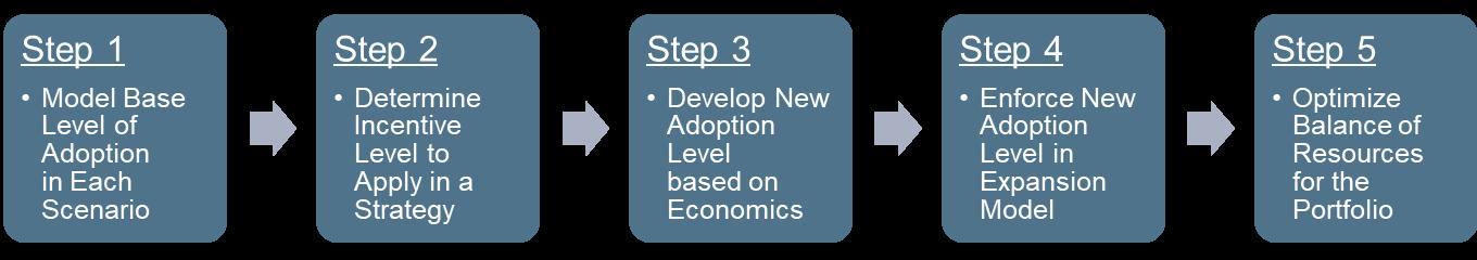
Base, moderate and high penetration levels for DG resources were determined using an adoption curve approach. The approach used is similar to NREL’s Distributed Market Demand Model, which simulates potential adoption of a given resource as a function of the number of payback years. Factors specific to each scenario and strategy combination were fed into a TVA-developed DG model to create a unique adoption level for each resource for the 20-year
planning horizon. Further details about this innovative modeling approach can be found in Appendix C: Distributed Generation Methodology.
The narratives supply the roadmap for designing the strategies, and a consistent incentive structure provides the mechanism for promoting resources in each strategy. The Strategy Design Matrix (Figure F4) brings the two together, showing how resources are being promoted across the strategies. Finally, innovation in DG modeling allows TVA to evaluate how a combination of DG and utility-scale resources might ultimately impact future resource portfolios.
The capacity expansion plans are shown below by strategy. The capacity graphics show the total
Total Capacity Expansion Plans:
capacity grouped by resource type (i.e., nuclear, hydro, coal, etc.) over the planning horizon. The capacity is in gigawatts, which is 1,000 megawatts, and is based on the summer net dependable capacity value, which is the amount of capacity that TVA plans to have available to meet summer peak firm requirements
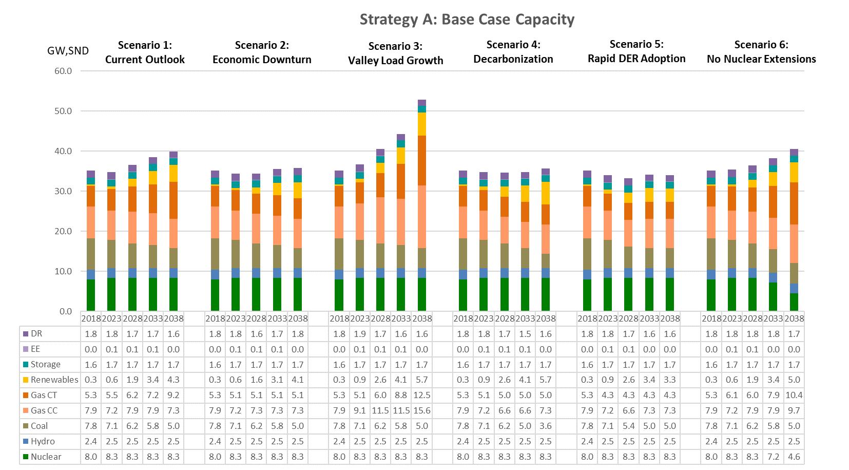
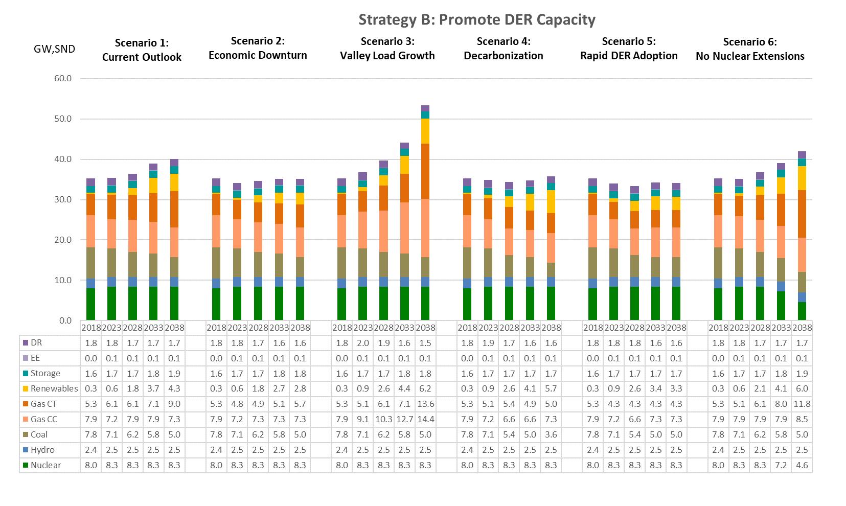
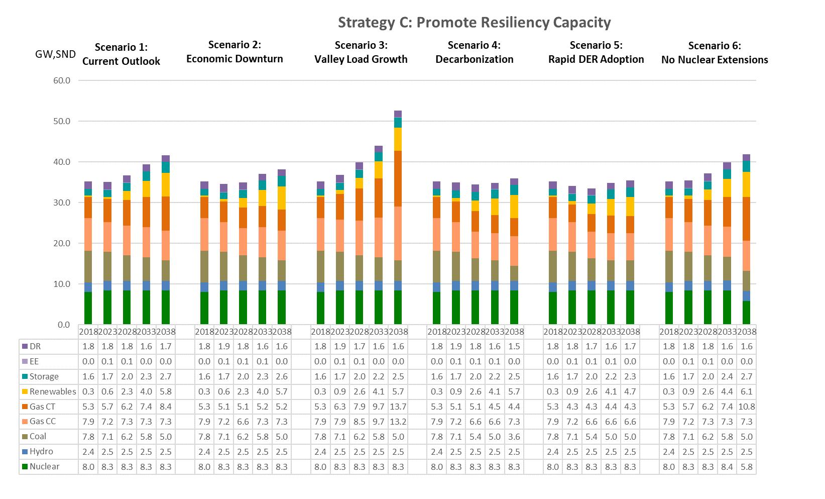
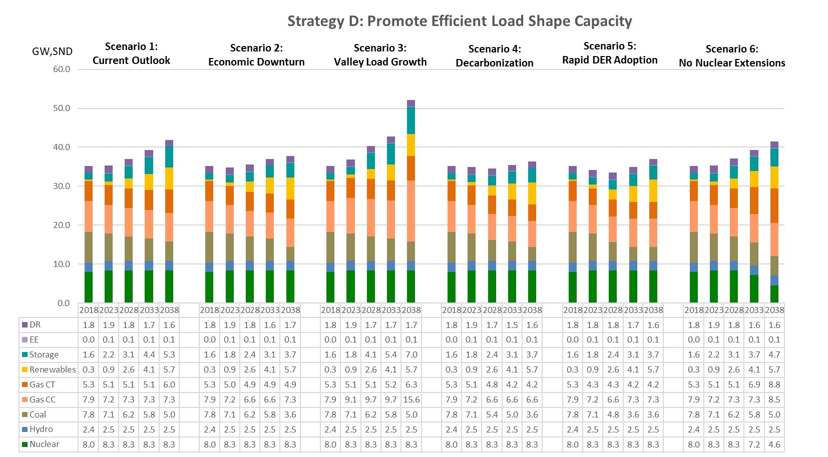
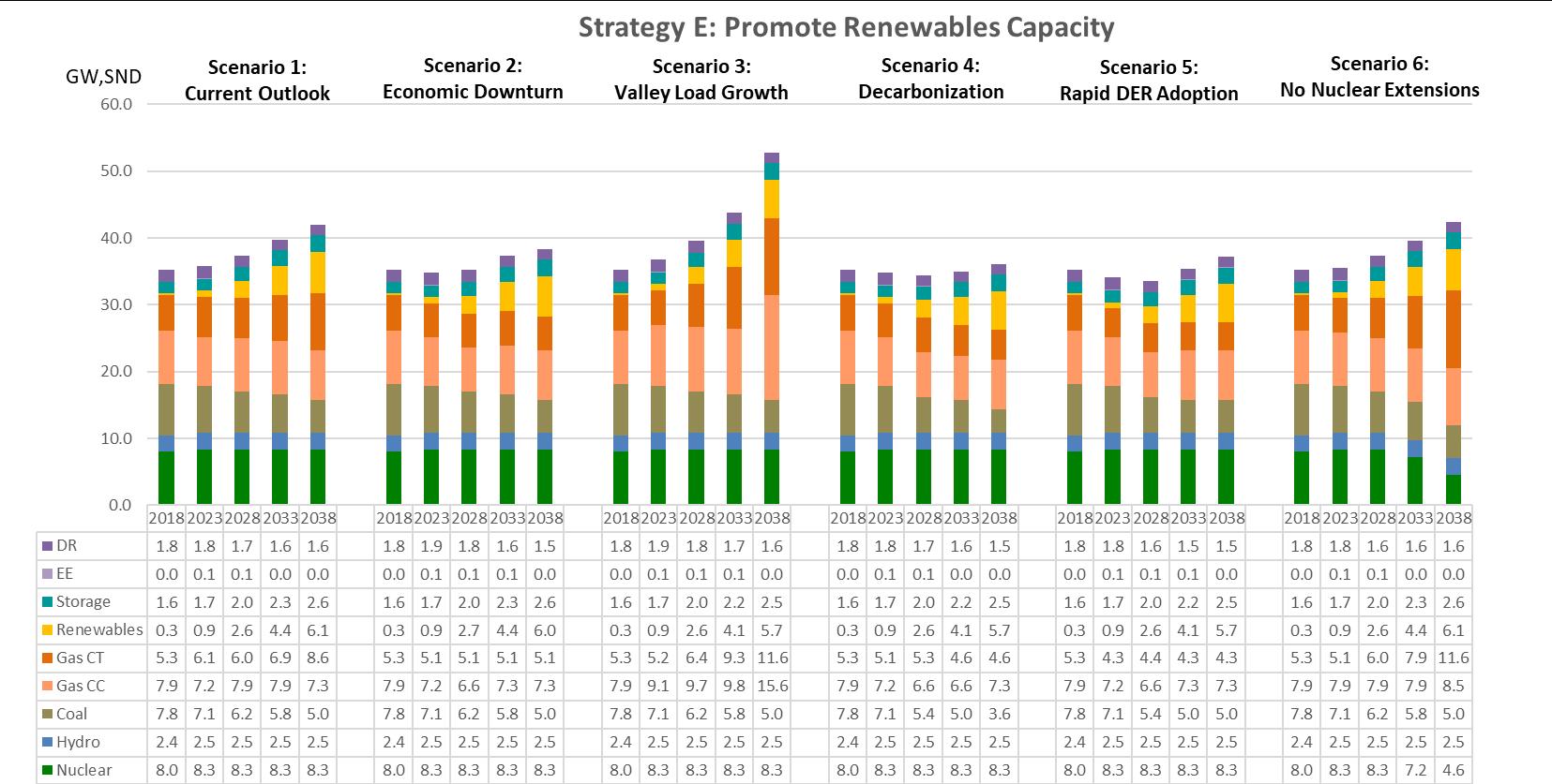
The total energy charts provided below correspond to the capacity expansion plans shown in the previous
section. The energy charts show total energy grouped by resource type (i.e., nuclear, hydro, coal, etc.) over the planning horizon and are in terawatt hours, which is a 1,000 gigawatt hours.
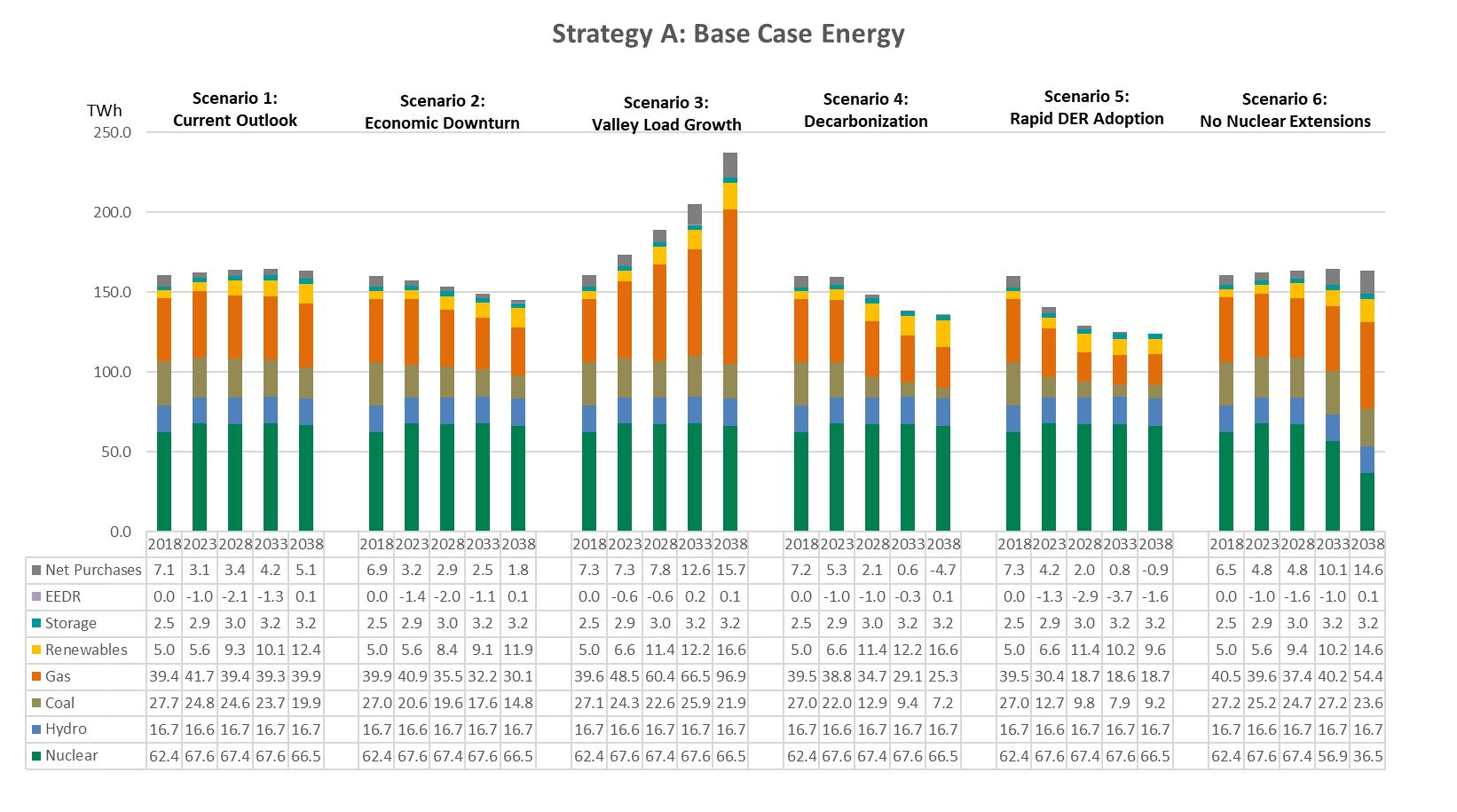
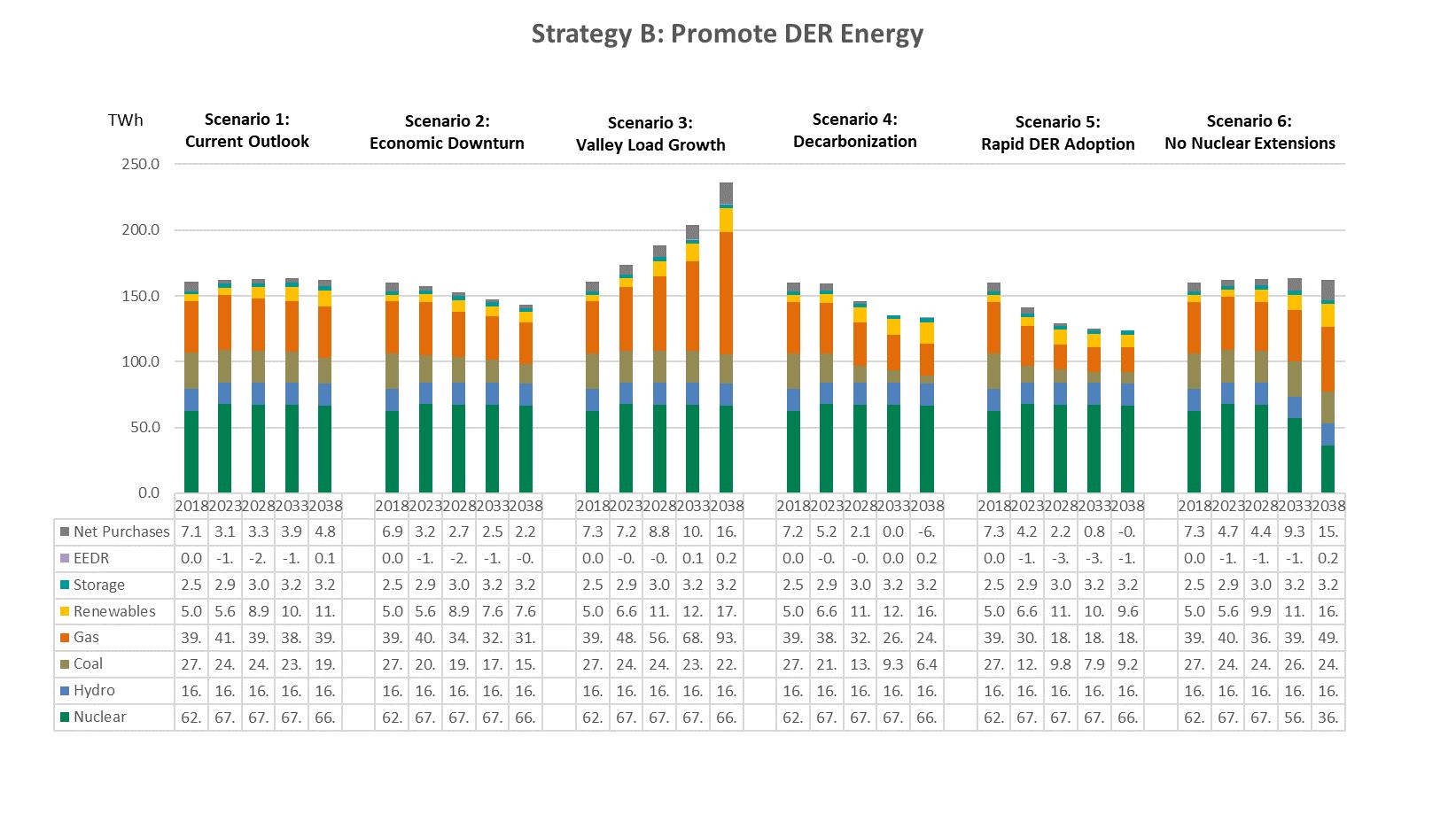
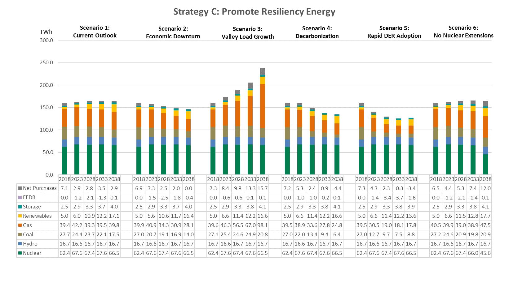
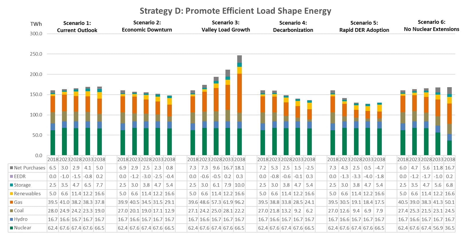
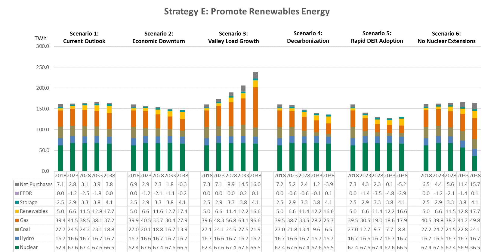
The reserve margin charts provided below for summer and winter correspond to the capacity expansion plans shown in the previous section. TVA established reserve margin targets of 17 percent for summer and 25 percent for winter for this IRP.
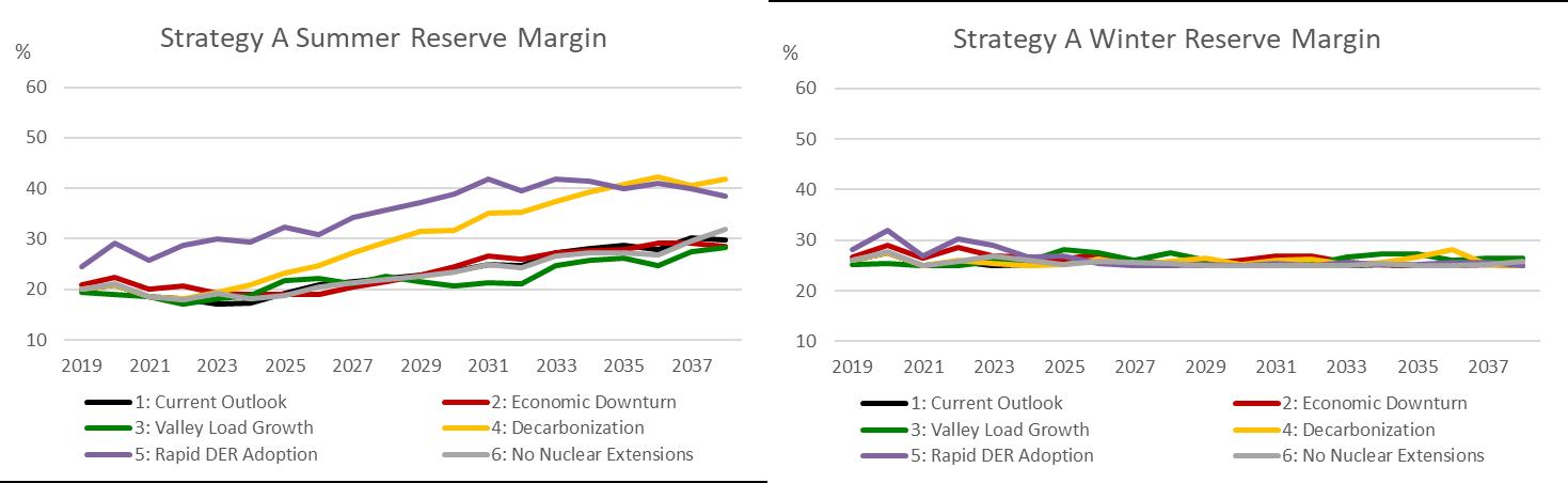
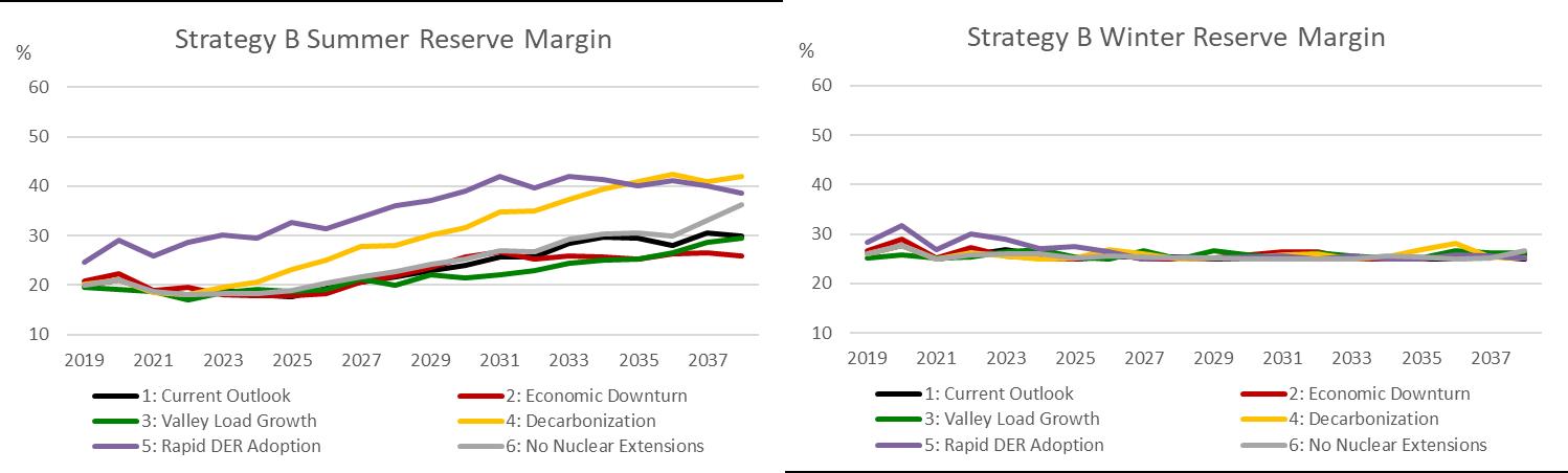
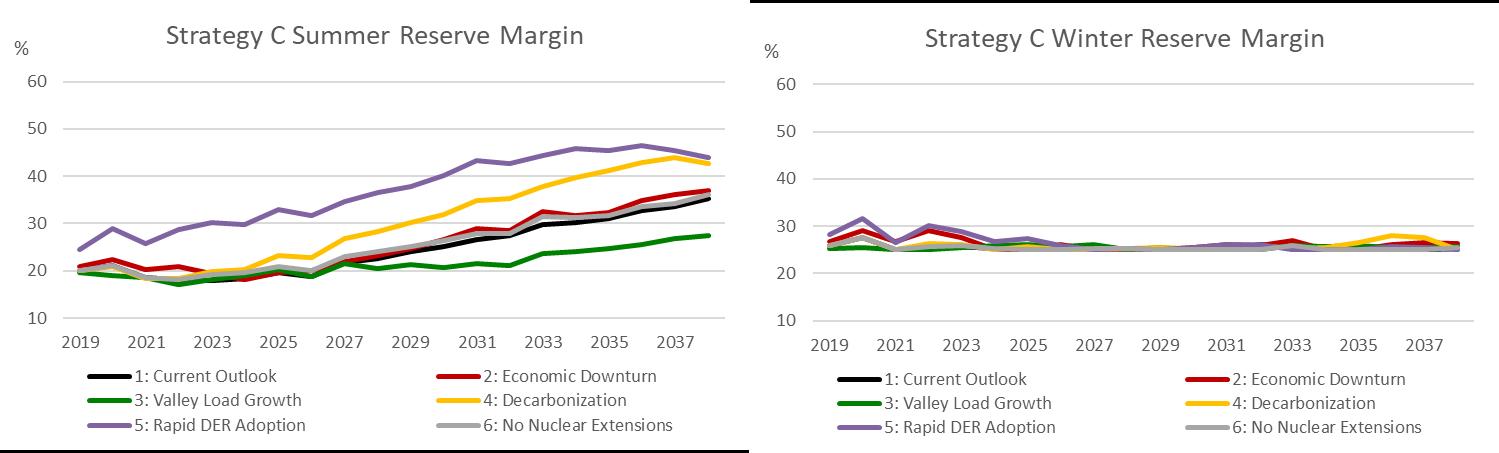
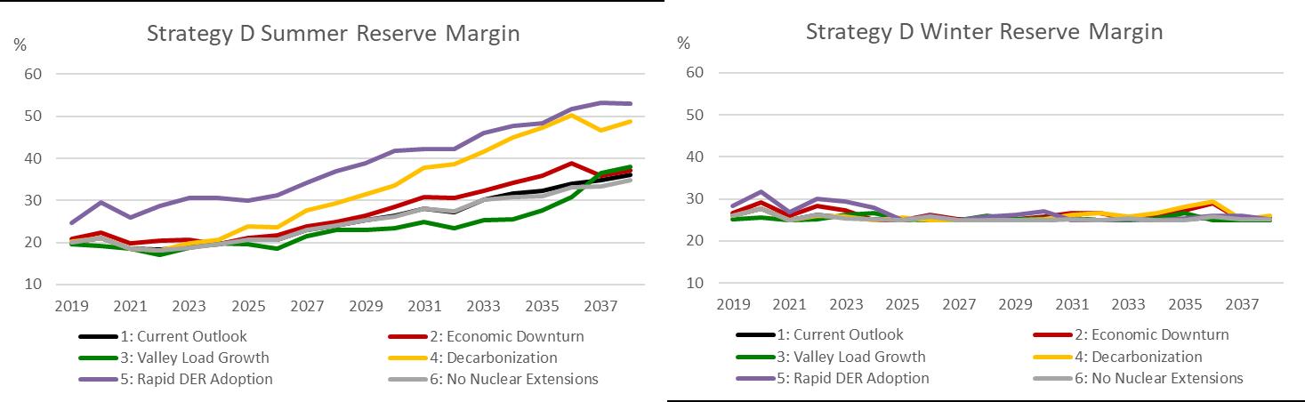
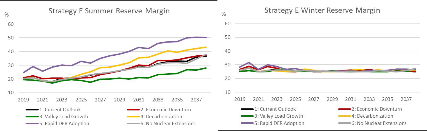
The total capacity additions on a year by year basis are shown below for the five strategies in each scenario. Scenarios are represented by number (1 to
6) and strategies by letter (A to E) The data is shown in summer net dependable gigawatts (SND GW) and is grouped by resource type (i.e., nuclear, hydro, coal, etc.) over the planning horizon.
Appendix H - Stochastic Results for Cost Metrics
HAppendix H - Stochastic Results for Cost Metrics
For the 2019 IRP, the three primary cost metrics selected are Present Value of Revenue Requirements (PVRR), System Average Cost and total resource cost (TRC) The charts in this section
show the expected case (where colored bars meet) and the range of results around the expected case based on stochastic variation of the key planning variables for each portfolio

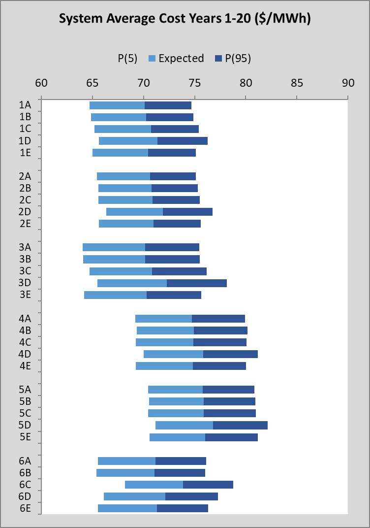
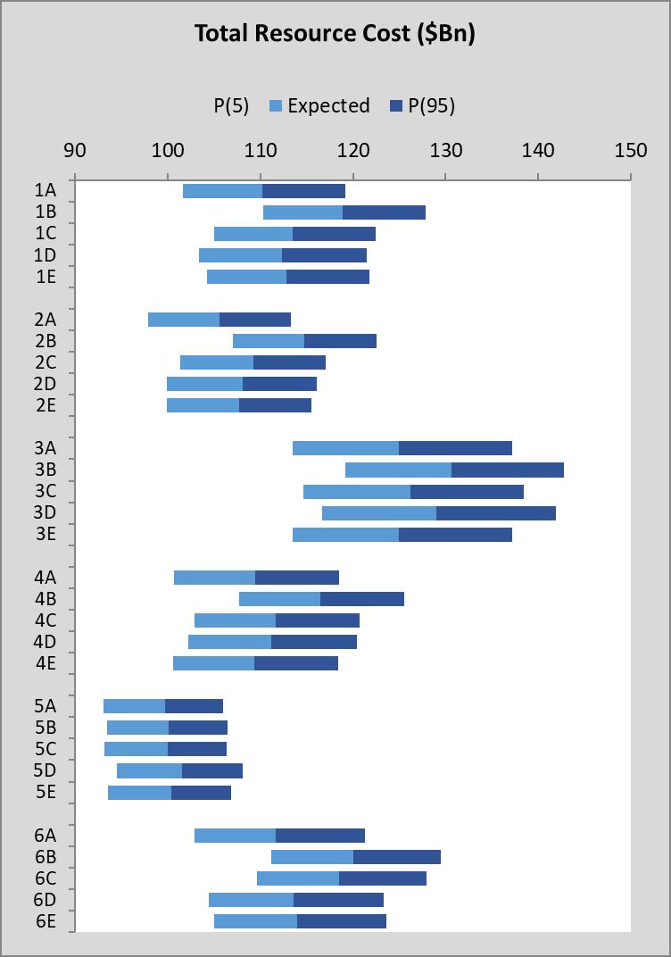
This page intentionally left blank.
In developing the criteria for the environmental impact metrics, TVA wanted to create a set of metrics representative of the trade-offs between energy resources rather than identifying a single resource with “best” environmental performance. Consideration of air impacts, water consumption, waste production and land use in the IRP scorecard, coupled with the broader qualitative assessment of anticipated environmental impacts in the EIS, allowed TVA to make a robust comparison of the environmental footprint of the planning strategies that informed the selection of the recommended strategy.
For the 2019 IRP, five environmental impact metrics for air, water, waste and land use were selected.
CO2 Metric Results:
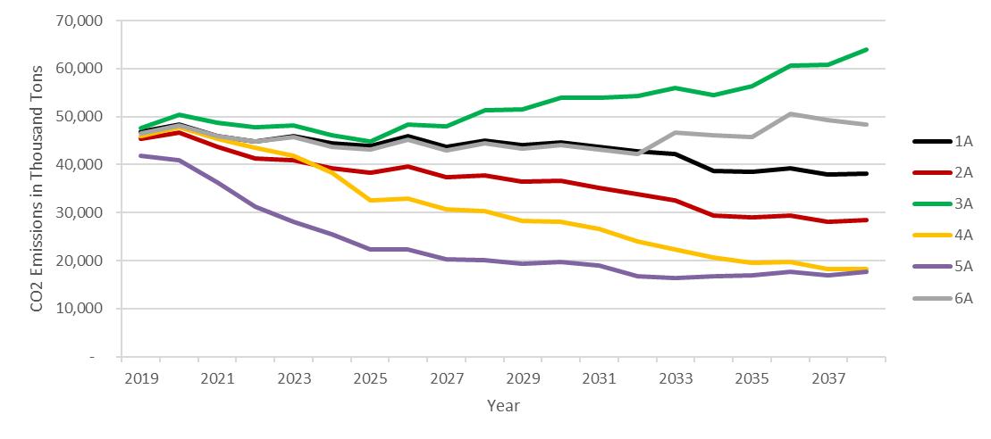
Strategy A: Base Case
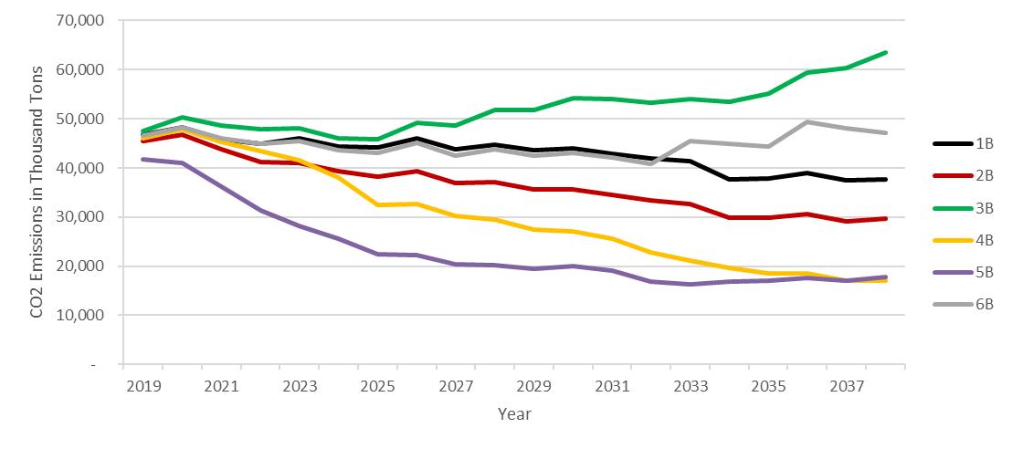
Strategy B: Promote DER
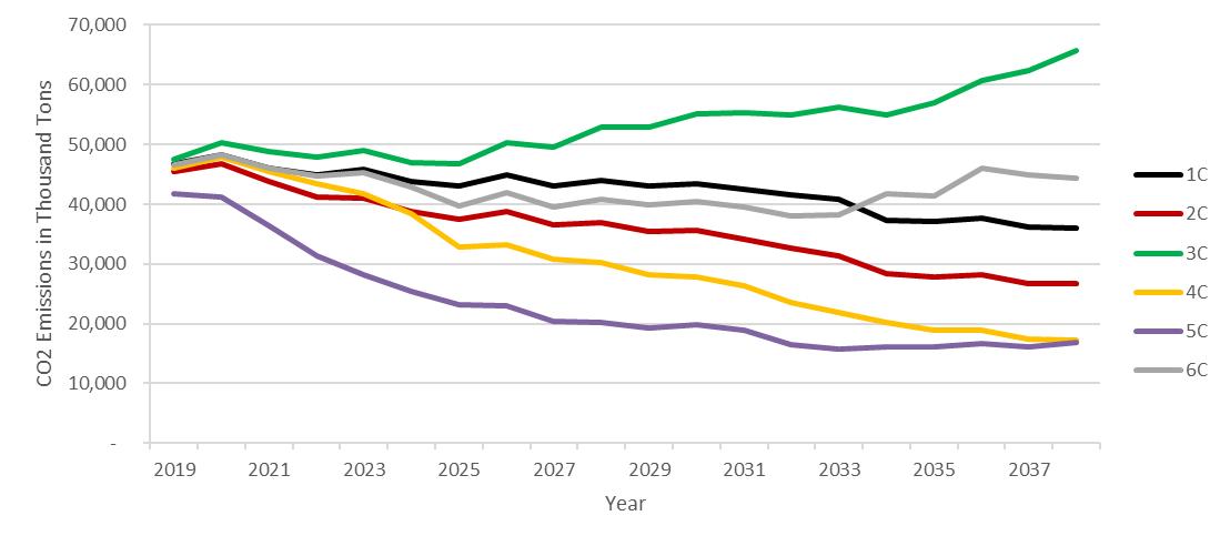
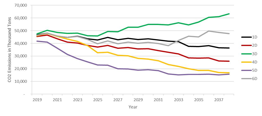
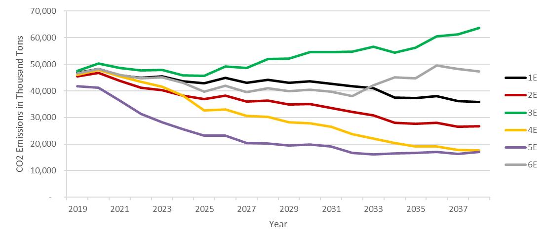
CO2 Intensity Metric Results:
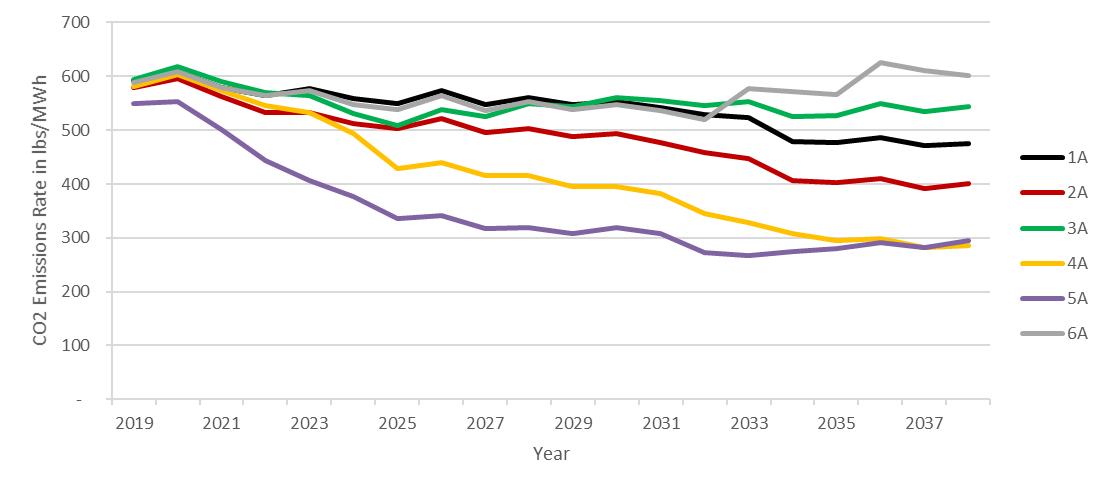
Strategy A: Base Case
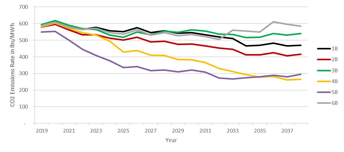
Strategy B: Promote DER
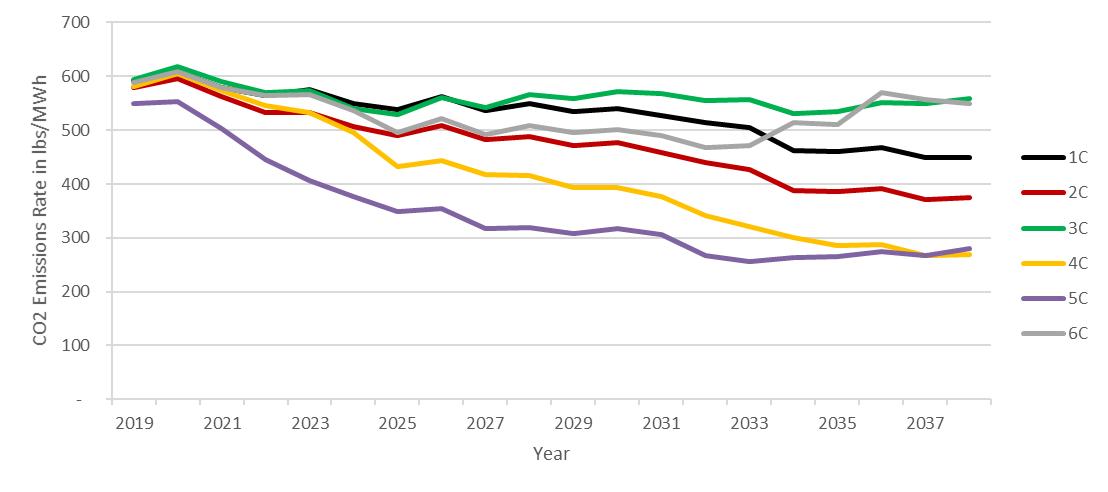

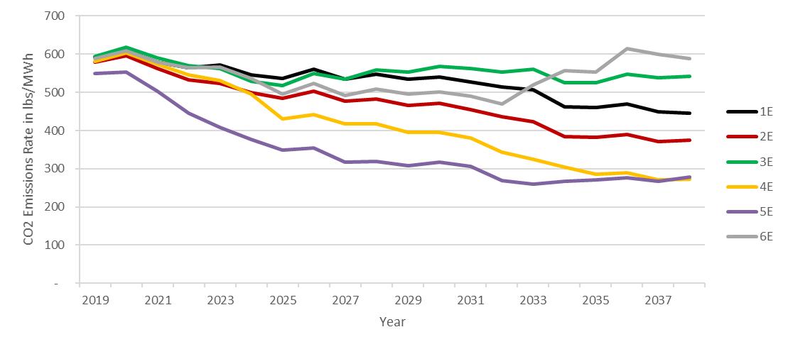
Strategy E: Promote Renewables
Water Consumption Metric Results:
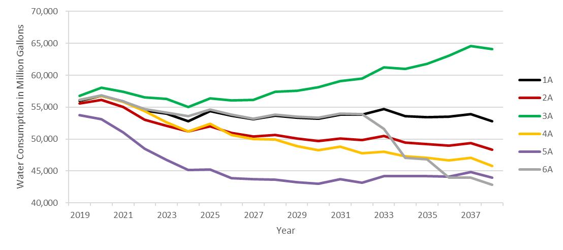
Strategy A: Base Case

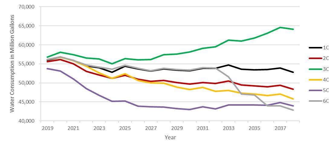

Strategy D: Promote Efficient Load Shape

Strategy E: Promote Renewables
Waste Metric Results:
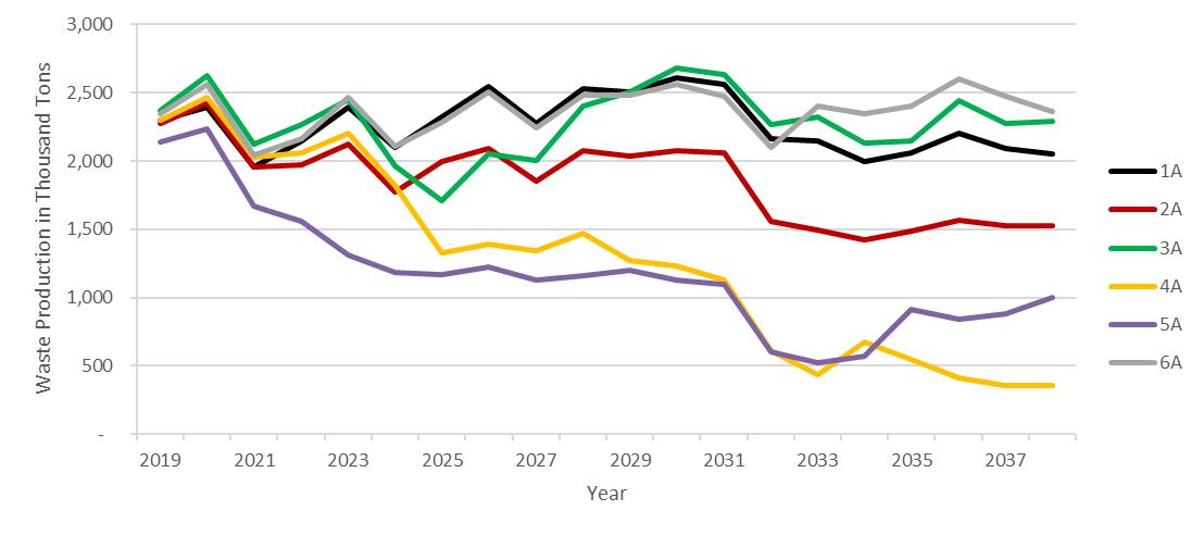
Strategy A: Base Case
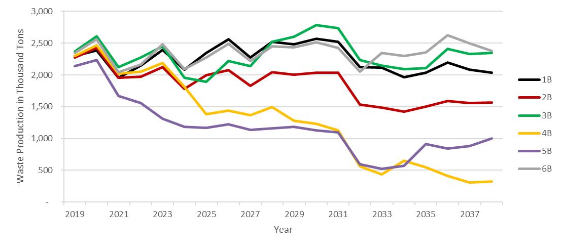
Strategy B: Promote DER
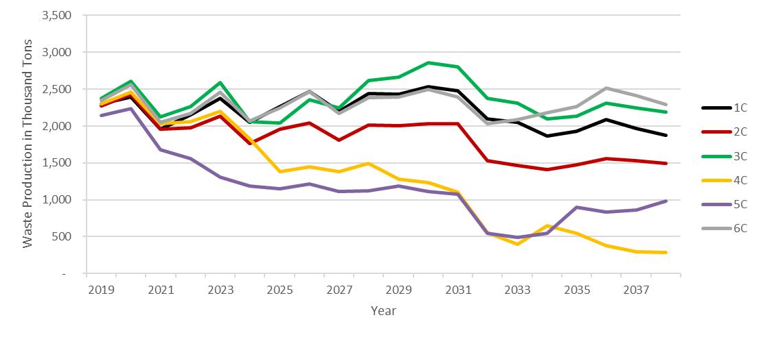
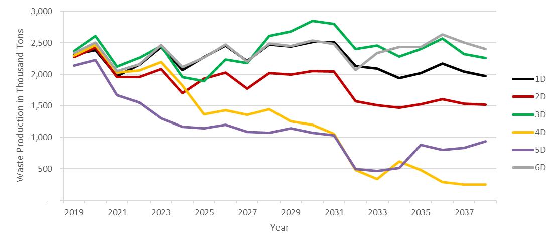
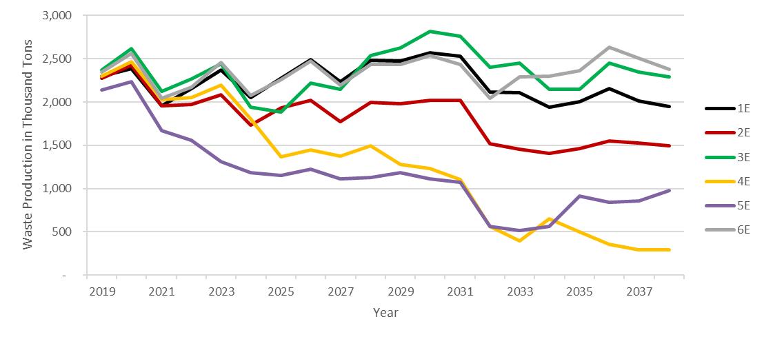
Strategy E: Promote Renewables
Land Use Metric Results:
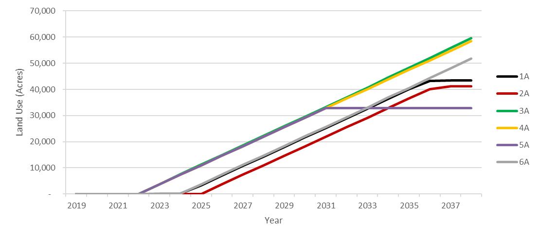
Strategy A: Base Case
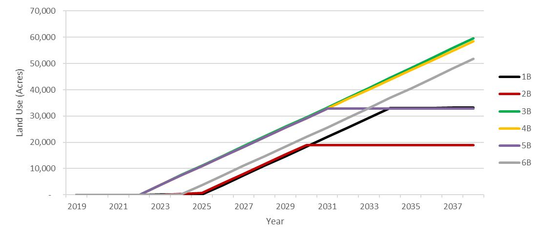
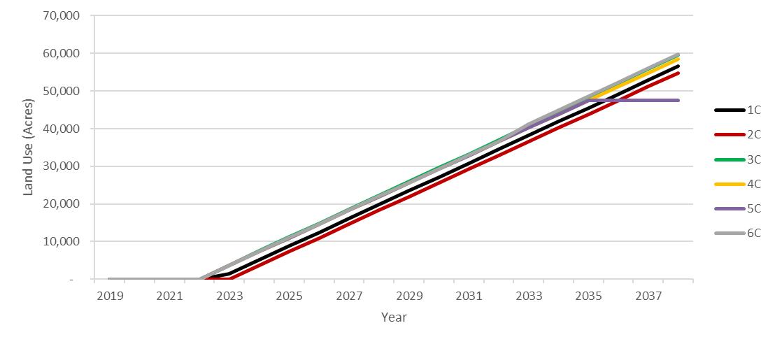
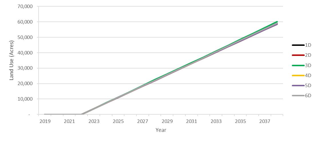
Strategy D: Promote Efficient Load Shape
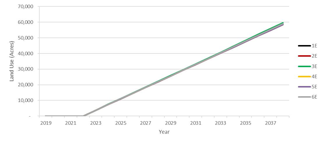
Strategy E: Promote Renewables
Stochastic analysis was used to determine potential ranges of results for the Air and Water Impact metrics.
The charts in this section show the expected case (where colored bars meet) and the range of results around the expected case based on stochastic variation of the key planning variables for each portfolio
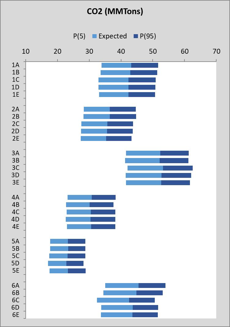
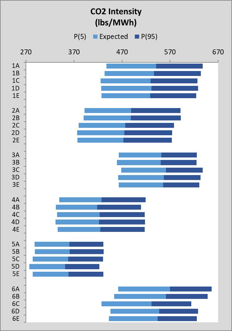
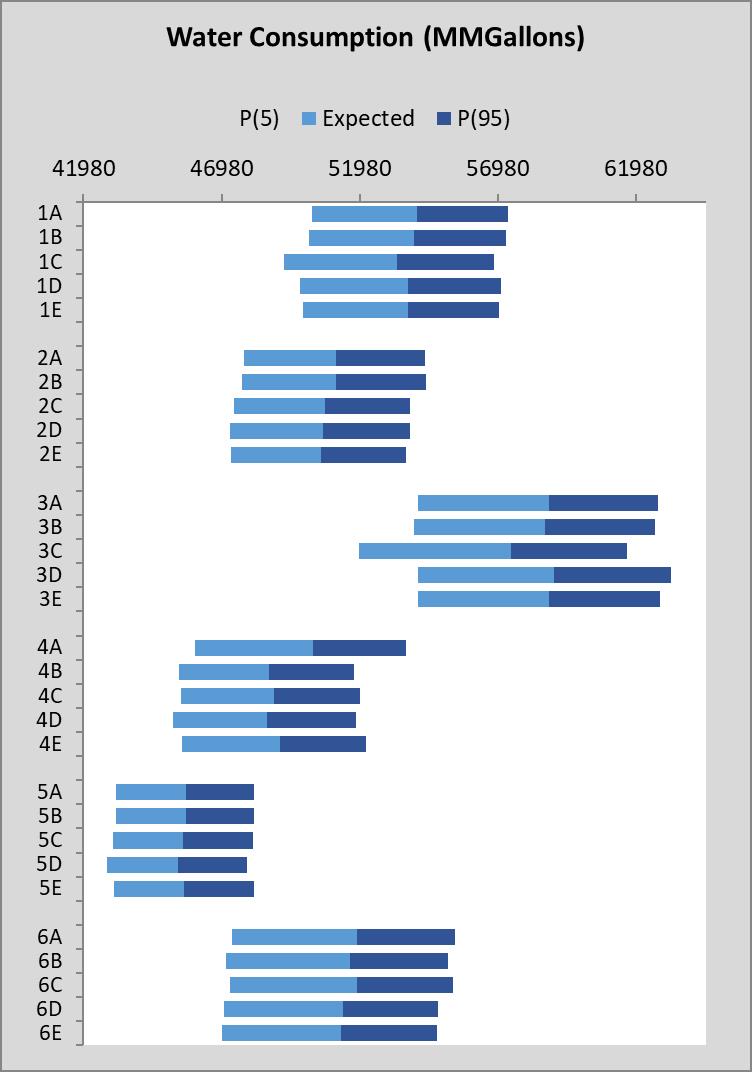
This page intentionally left blank.
Because the TVA Act promotes agricultural and industrial development as a core TVA responsibility, the economic well-being of Tennessee Valley (hereafter Valley) residents has been part of the TVA’s mission since 1933. In keeping with TVA’s core mission, the IRP scorecard incorporates economic impact metrics for all portfolios, covering each scenario and strategy combination under consideration. Real per capita income and total nonfarm employment within the Valley are calculated in order to assess the relative impact of each strategy on the general economic conditions in the TVA region. This appendix describes the process used to calculate these two metrics. It also includes supporting information related to manufacturing employment and total Valley population projections
The U.S. Bureau of Economic Analysis provides a broad measure of real per capita income that reflects not just wage income but total compensation, such as employer contributions to health insurance and retirement accounts. Additionally, it includes other income sources, such as dividends and transfer payments. Thus, real per capita income provides a single metric that broadly reflects the general economic well-being of Valley residents and is readily
understandable and relatable. It also reflects the net effect of each strategy’s change in expenditures and electricity bills. Increases in TVA expenditures on labor, equipment, fuels, and construction materials stimulate the economy. At the same time, increases in consumers’ electricity bills required to fund those operations and construction activities reduce consumers’ discretionary income. Discretionary income reflects the share of income left over after paying for necessities such as rent (or mortgage payment), healthcare, food, clothing, transportation, and energy costs (including utilities). Lower discretionary income translates into reduced consumer purchases on other goods and services in the TVA region. Because strategies that involve increasing in-Valley expenditures tend to require higher electricity bills, their impacts tend to be offsetting.
The PI+ Model by Regional Economic Models, Inc., hereafter referred to as REMI, is used to model the multiplier effects of each strategy’s expenditures that stimulate the regional economy and its electrical bills that dampen it. REMI is a general equilibrium model used by TVA for over 15 years and is currently in use by over 100 universities, state and local governments, utilities, and consulting firms throughout the U.S. and Europe. TVA’s model has been tailored to the TVA region by county and optimized to capture the interindustry and inter-regional linkages with surrounding counties and the rest of the United States. As shown in Figure J-1, the “direct effects,” i.e., changes in TVA expenditures and retail electricity bills, are input into REMI, which capture any multiplier effects and interactions within the regional economy.
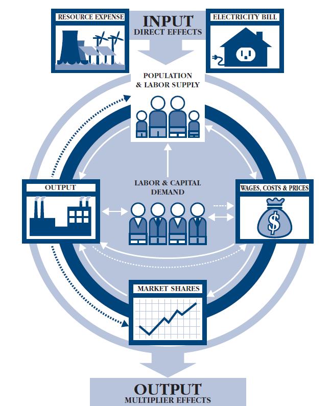
Strategy A of each scenario serves as the Base Case, so each strategy within each scenario is compared to Strategy A. Thus, increases in expenditures are only entered into REMI to the extent that they exceed Strategy A expenses. In this way REMI outputs are the impact on real per capita income relative to the Base Case in each scenario.
Within a scenario, each strategy has a different annual revenue requirement needed to fund its construction, generation, and energy efficiency programs. The difference between the Base Case and the revenue requirements of other strategies are modeled as changes in the electricity bill for
residential, commercial, and industrial customers. Ultimately, ratepayers must fund any increase in TVA expenditures.
While increases in the revenue requirements of a strategy tend to reduce consumers’ ability to purchase goods and services, an increase in TVA expenditures stimulates economic activity, at least to the extent such goods and services are purchased within the TVA region. Expenditures that are almost exclusively sourced outside the TVA region, such as fuel or purchased wind power from the Midwest, are excluded from TVA region expenditures.
Because not all types of expenses have identical economic impacts, REMI is used to separately model the impact of renewable construction, non-renewable
construction, non-fuel operation and maintenance (O&M), and energy efficiency expenses. In this way REMI identifies the ability of the TVA regional economy to supply the necessary inputs and to what extent they must be sourced outside the region. Because most new non-renewable construction expenses are likely to be natural gas-fired power plants, REMI’s custom construction industry for natural gas-fired power plants model is incorporated into the analysis. Similarly, since most new renewable construction in the TVA region will be solar installations, REMI’s custom industry solar plant construction model is used. This delineation between types of construction expenditures enhanced the accuracy of the results, reflecting the nature of expansion in each portfolio
While there are ongoing national codes and standards that increase energy efficiency, TVA implements programs that expedite the adoption of energy efficiency measures that are over and above the minimum required. The economic impact of TVA investments in energy efficiency programs is modeled as 7.52 new jobs in the TVA region for each $1 million spent in 2018-inflation-adjusted dollars. Of the jobs created, 20 percent fall within the utility industry, 20 percent in the construction industry, and 60 percent in professional/scientific employment categories. All differences from the Base Case are annual values, so changes in per capita income are generated by year. In economics, a real value of a good or other entity has been adjusted for inflation, enabling comparison of quantities as if prices had not changed. Changes in real terms therefore exclude the effect of inflation. In contrast with a real value, a nominal value has not been adjusted for inflation, and so changes in nominal value reflect at least in part the effect of inflation. The real per capita income output models the trajectory of economic impacts over time. In order to rank and compare alternative strategies, the present value of the changes in per capita income is evaluated by first deflating nominal per capita income values within each scenario by its projected consumer price index
(hereafter CPI) over the 2019 to 2038 period to place the values in constant 2018-dollars, and then applying a 2 percent discount rate across the 20-year-horizon to account for the time value of money. REMI also accounts for the inflationary/deflationary impacts of alternative strategies on electricity prices within the Valley on that scenario’s CPI. Average annual changes in non-farm employment are presented as well. In order to obtain further insight, this appendix also reports projected changes in manufacturing employment and total service-area population.
These results are based on the Present Value of Revenue Requirements (PVRR) over the 20-year study period (2019-2038). The 2019 IRP also considers Total Resource Cost (TRC) which takes into account the net participant cost borne by the end use customer. Consideration of these costs could also impact real per capita income and employment results, beyond PVRR-based impacts summarized in this appendix.
Table J-1 provides changes in the TVA region’s real per capita income caused by each strategy. The difference in all scenarios across all strategies is relatively small. From 2019 to 2038, the average percentage change in real per capita income ranged from -0.04 percent to +0.01 percent. The results are expected to be small for several reasons. First, TVA revenue is a small percentage of the total TVA region economy. In 2019, TVA revenues are expected to approach $11 billion, but the entire TVA region economy amounts to roughly $440 billion. Second, the proposed strategies result in relatively similar approaches to supplying the region’s power needs, and generally do not dramatically change TVA revenue requirements in a given year Changing from one approach to another or employing a combination of strategies should not result in significant impacts on the economy as a whole.
2019-2038
Across the six scenarios, there are meaningfully different assumptions about economic conditions nationwide that impact the TVA region’s standard of living, especially across Scenarios 1 – 4 Real per
No
Table J-2 presents the average change in the TVA region’s total non-farm employment due to each strategy. Once again, the difference in all scenarios across all strategies is quite small. From 2019 to 2038
capita incomes (hereafter PCI) are not, however, comparable across scenarios because the varying scenario assumptions generally overwhelm strategydriven impacts.
the average percentage change in non-farm employment ranges from 0.00 percent (actually0.005 percent) to +0.11 percent In a region with an employment base of roughly 4.4 million, these
investment changes are not of sufficient magnitude to substantially move the needle. Additionally, increases in total employment can occur in conjunction with declines in manufacturing employment (which generally possess higher average wage rates than in non-manufacturing sectors) and more than proportionate increases in population, suggesting that
migration into the Valley may more than offset any resulting increase in employment in some cases. Resulting labor force participation rates, unemployment rates, and income on a real per capita basis may not materially improve from Base Case conditions
Table J-3 presents the average change in the TVA region’s manufacturing employment due to each strategy. The differences in all scenarios across the strategies are modest. From 2019 to 2038, the average percentage change in manufacturing employment range from -0.03 percent to +0.08 percent. In absolute terms this translates into a decline of 150 manufacturing jobs in one of the No Nuclear Extensions cases to a gain of over 400 manufacturing jobs in one of the Rapid DER Adoption cases. Manufacturing employment generally
increases (or does not decline much) in the Promote DER strategy cases, as these cases generally entail the smallest relative change in TVA revenue requirements. The largest upside in employment, either total non-farm or manufacturing, occurs in the Rapid DER cases. This scenario assumes that a technological leap forward in DER technology would drive gains in labor demand as the resulting energy cost savings boosts discretionary income, thereby stimulating spending on other goods and services.
J-4
The differences in all scenarios across the strategies tend to parallel the changes in employment described above. From 2019 to 2038, the average percentage change in population ranges from -0.02 percent to +0.10 percent In absolute terms, this ranges from a decline of about 1,900 people in one No Nuclear Extensions case to a gain of 10,720 in the Rapid DER Adoption case. Once again, the largest increases in population occur in the Rapid DER Adoption cases, though it appears as though the nonfarm employment gains described above are generally matched by proportionate increases in population (accounting for typical household size of roughly 2.42 persons per household over this same time period).
The Current Outlook scenario reflects TVA’s expected Base Case assumptions with respect to the general state of the economy and power markets. Table J-5 below depicts the cumulative Revenue Requirements (RR, i.e. the change in electricity cost for each strategy relative to the Base Case) in proportion to the cumulative In-Valley capital expenditures, fixed O&M spending, and spending on energy efficiency programs within each strategy, all in 2018-inflationadjusted dollars.
*all values in Mil. 2018-$
Note that Strategy B (Promote DER) reflects the smallest increase in RR, both in absolute terms and relative to capital, fixed O&M, and EE expenditures
among the various strategies. An alternative way to think about this is that any change in TVA’s revenue requirements impacts ALL customers via higher
electricity costs, whereas a change in program spending on DER, EE, and renewable programs directly impacts program participants by lowering their electricity costs. However, the indirect impacts
reduced electricity sales on the part of TVA reduce TVA’s variable costs, but do not necessarily lower TVA’s fixed costs (at least in the short-run), which must now be spread across a smaller sales base.
In the Current Outlook scenario, Strategy B, Promote DER, is the most beneficial from the perspective of maximizing PCI; however, the resulting change in PCI is modest at roughly $1 per person per year, or $20 over the 2019 to 2038 period (in 2018 $)
The Economic Downturn scenario models a world in which economic growth stagnates and underlying inflation escalates In this case, none of the
alternative strategies translates into an increase in PCI, though the strategy with the smallest increase in RR (2B), or smallest ratio of RR change to total expenditure change (2E), translates into the least negative impact on PCI. (See Table J-6 and Figure J-
3) Given the relatively weaker overall state of the economy in this scenario, an increase in electricity costs of any magnitude exerts a negative impact on economic well-being across the Valley.
The Valley Load Growth Scenario models an environment of sustained, robust economic growth and growing demand for power. Once again, the optimal outcome in this scenario occurs under Strategy B, Promote DER. Under this strategy, TVA’s
revenue requirements actually decline over the 2019 – 2038 timeframe This is accompanied by a slight increase in overall spending on in-Valley DER and EE programs. (See Table J-7 and Figure J-4) The second most attractive alternative, albeit with a decline in PCI, is Strategy E – Promote Renewables, as it reflects the smallest absolute increase in revenue requirements among the three remaining cases.
The Decarbonization Scenario models a regulatory environment in which there are significant carbon
taxes that impact the relative efficiency of alternative strategies. These taxes translate into generally slower economic growth, although not as severe as in the Economic Downturn case.
*all values in Mil. 2018-$
In the scenario, Strategy B – Promote DER, provides a positive boost to PCI as shown in the following figure. It reflects the smallest level of increased revenue requirements yet the second highest
program spending level of all the Decarbonization cases. This translates into a modest increase in average PCI over the forecast period (See Table J-8 and Figure J-5)
The Rapid DER Scenario models a world in which there is a dramatic leap forward in technology which drives a strong shift toward distributed energy resources, both from a generation, energy storage, and efficiency perspective Given the nature of the material technological shift in this scenario, none of the four strategies improves upon the Base Case
results from an economic impact perspective, likely because with a rapid private sector shift in DER investment, any incremental TVA expenditures do not have as significant an impact on the Valley economy However, Strategy B, which entails the smallest increase in RR, translates into the smallest absolute decline in PCI across these strategies. (See Table J-9 and Figure J-6)
The No Nuclear Extensions Scenario models a world in which TVA is unable to relicense its Browns Ferry units, and must rely upon investments in small modular reactors and increased utility and/or customer-owned supply options As a result of the
increase in generation costs in this Base Case, PCI generally declines in all these cases However, Strategy B does reflect a small decrease in RR, translating into a slight rebound in PCI relative to the Base Case. Given the material shortfall in TVA generation due to the loss of a major base load nuclear resource, the paybacks to a small increment of DER spend is positive. (See Table J-10 and Figure J-7)
There are multiple approaches to meeting the TVA region’s power needs. This analysis compared the economic impact of alternative strategies to that of the Base Case for each respective scenario. Each strategy involved changing the level of in-Valley expenditures and the magnitude of electricity bills required to satisfy each strategy’s funding needs. Using REMI’s PI+ general equilibrium model tailored to the TVA service territory, the impact on real per capita income of alternative strategies for meeting power demand was evaluated. By using custom industry models and base REMI capabilities, the impacts of different types of expenditures (e.g., renewable construction, non-renewable construction, non-fuel O&M) were modeled explicitly.
Under most scenarios Strategy B, Promote DER, generated the largest gains in real per capita income over and above the Base Case These programs generally entailed the smallest change in RR
However, Strategy B results in the highest Total Resource Cost due to the increased net participant cost from distributed resources not directly reflected in the estimation of the economic impact metrics.
Overall, the impact of all alternative strategies on real per capita income was very small. Across all scenarios and strategies the average percentage change in real per capita income from 2019 through 2038 ranged from -0.04 percent to 0.01 percent. The
present value of the stream of annual differences is small as well. The inherent forecast uncertainty in the economic projections alone will likely far exceed these magnitudes of change across the various strategies. Any material increase in program spending on TVA’s part, while generating spin-off economic impacts, also entails increased RR to fund it. This results in secondary impacts on regional inflation, population migration patterns, and manufacturing employment, which tend to mitigate the resulting impacts on inflation-adjusted (real) per capita income for the region.