
Microsoft Excel 2013 Chapter 2 – Lab Test A Performing Sales Analysis
Purpose: To demonstrate the ability to enter and copy formulas, and apply formatting to a worksheet.
Problem: You are the accountant for a collectibles business that has store locations all throughout the state. You are trying to determine if stores are meeting their sales quotas. You know the sales amount, returns amount, and sales quota. You will calculate the rest using functions.
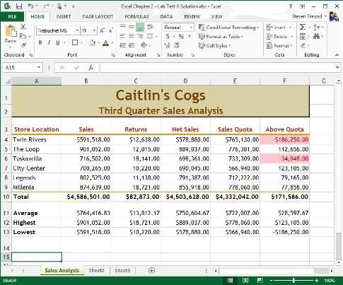
Instructions: Perform the following tasks to create the worksheet shown in Figure E2A - 1.
1. Enter and format the worksheet title Caitlin’s Cogs and worksheet subtitle Third Quarter Sales Analysis in cells A1 and A2. Apply the Berlin theme to the worksheet. Apply the Title cell style to cells A1 and A2. Change the font size in cell A1 to 28 points. Merge and center the worksheet title and subtitle across columns A through F. Change the background color of cells A1 and A2 to Tan, Accent 2, Lighter 40%. Change the font color of cells A1 and A2 to Orange, Accent 1, Darker 50%. Draw a thick box border around the range A1:A2.
2. Change the width of columns A through F to 15.00 points. Change the heights of row 3 to 33.00 points and row 11 to 30.00 points.
3. Enter the column titles in row 3 and row titles in the range A10:A13, as shown in Figure E2A - 1.Center the column titles in the range A3:F3. Apply the Heading 1 cell style to the range A3:F3. Apply the Total cell style to the range A10:F10. Bold the titles in the range A11:A13. Change the font size in the range A3:F13 to 12 points.
4. Enter the data for the Store Location (A4:A9), Sales (B4:B9), Returns (C4:C9), and Sales Quota (E4:E9) columns using the column info from Figure E2A - 1.
5. Use the following formulas to determine the Net Sales in column D and the Above Quota in column F for the first store location. Copy the two formulas down through the remaining store locations.
a. Net Sales (cell C4) = Sales – Returns
b. Above Quota (F4) = Net Sales – Sales Quota
6. Determine the totals in row 10.
7. Determine the average, maximum, and minimum values in cells B11:B13 for the range B4:B9, and then copy the range B11:B13 to C11:F13.
8. Format the numbers as follows: (a) assign the Currency style with a floating dollar sign to the cells containing numeric data in the ranges B4:F4 and B10:F13, and (b) assign a number style with two decimal places and a thousand’s separator to the range B5:F9.
9. Use conditional formatting to change the formatting to Light Red Fill with Dark Red Text in any cell in the range F4:F9 that contains a value less than 0.
10. Change the worksheet name from Sheet1 to Sales Analysis and the sheet tab color to the Orange standard color. Change the worksheet header with your name, course number, and other information as specified by your instructor.
11. Spell check the worksheet. Preview and then print the worksheet in landscape orientation. Save the workbook using the file name, Excel Chapter 2 – Lab Test A.
12. Print the range A3:F13. Print the formulas version on another page. Close the workbook without saving the changes. Submit the assignment as specified by your instructor.
Microsoft Excel 2013 Chapter 2 – Lab Test B
Performing Payroll Analysis
Purpose: To demonstrate the ability to enter and copy formulas, and apply formatting to a worksheet.
Problem: You work for Timothy’s Technology Repair. You are in charge of maintaining the payroll for the store. You have been given the basic information about the employees and will use functions to calculate the remaining payroll information.
Instructions: Perform the following tasks to create the worksheet shown in Figure E2B - 1.
1. Enter and format the worksheet title Timothy’s Technology Repair and worksheet subtitle Payroll Summary in cells A1 and A2. Apply the Retrospect theme to the worksheet. Apply the Title cell style to cells A1 and A2. Change the font size in cell A1 to 28 points. Merge and center the worksheet title and subtitle across columns A through G. Change the background color of cells A1 and A2 to Brown, Accent 4, Lighter 60%. Draw a thick box border around the range A1:A2.
2. Change the width of column A to 18.71 points. Change the widths of columns B through G to 13.00 points. Change the heights of row 3 to 39.00 points and row 14 to 30.00 points.
3. Enter the column titles in row 3 and row titles in the range A13:A16, as shown in Figure E2B - 1. Center the column titles in the range A3:G3. Apply the Heading 3 cell style to the range A3:G3. Apply the Total cell style to the range A13:G13. Bold the titles in the range A14:A16. Change the font size in the range A3:G16 to 12 points. Center the range B4:B16.
4. Enter the data for the Employee, Dependents, Hourly Rate, and Hours Worked columns (A4:D12) using the column info from Figure E2B - 1.
5. Use the following formulas to determine the Gross Pay in column E, Taxes in column F, and Net Pay in column G for the first employee. Copy the three formulas down through the remaining employees.
a. Gross Pay (cell E4) = Hourly Rate * Hours Worked
b. Taxes (F4) = 20% * (Gross Pay – Dependents*24.36)
c. Net Pay (G4) = Gross Pay – Taxes
6. Determine the totals in row 13 for the range D13:G13.
7. Determine the maximum, average, and minimum values in cells B14:B16 for the range B4:B12, and then copy the range B14:B16 to C14:G16
8. Format the numbers as follows: (a) assign the Currency style with a floating dollar sign to the cells containing numeric data in the ranges C14:C16, E4:G4, and E13:G16 and cell C4; (b) assign a number style with two decimal places and a thousand’s separator to the ranges C5:C12, D4:D16, and E5:G12; and (c) assign a number style with zero decimal places to the ranges B4:B12 and B14:B16.
9. Use conditional formatting to change the formatting to white font on a blue standard background in any cell in the range D4:D12 that contains a value greater than 30.
10. Change the worksheet name from Sheet1 to Payroll Summary and the sheet tab color to the Blue standard color. Change the worksheet header with your name, course number, and other information as specified by your instructor.
11. Spell check the worksheet. Preview and then print the worksheet in landscape orientation. Save the workbook using the file name, Excel Chapter 2 – Lab Test B.
12. Print the range A3:E16. Print the formulas version of the sheet on another page. Close the workbook without saving the changes. Submit the assignment as specified by your instructor.
