Force Calibration Guidance for Beginners, Part 2
Effects of Impurities on the Freezing Plateau of the Triple Point of Water
Practitioner’s Perspective on the GUM Revision, Part 2: Examples and Resolutions to the Ballico Paradox
OCTOBER NOVEMBER DECEMBER
2022
DANISENSE

PRECISION CURRENT TRANSDUCERS

HIGH CURRENT CALIBRATION SERVICES


CURRENT INSTRUMENTATION AND CURRENT
HIGH
± 50A to ± 10000A DC/AC precision fluxgate current transducers for power measurement, battery test systems, high-stability power supplies, and current calibrations. • Current Ranges 50A ... > 10000A • Linearity Error down to 2 ppm • Very high absolute amplitude and phase accuracy from dc to over 1kHz • Low signal output noise • Low fluxgate switching noise on the pimary PRECISION
CALIBRATION
WWW.GMW.COM | INSTRUMENTATION FOR ELECTRIC CURRENT AND MAGNETIC FIELD MEASUREMENT
Your ability to deliver accurate and reliable measurements depends on the stability of your equipment, and your equipment depends on the accuracy and quality of its calibration. With over 25 years of calibration experience, GMW offers AC and DC NIST Traceable and/or ISO/IEC 17025:2005 Accredited* current calibration services for Current Transducers at our San Carlos, CA location and On-Site for minimal disruption of daily operations. Transducers manufacturers calibrated by GMW include, but not limited to, Danisense, LEM, GE, ABB, Danfysik, Hitec, AEMC, VAC, PEM, Yokogawa. * See gmw.com/current-calibration for Scope of Accreditation
1 Oct • Nov • Dec 2022
Volume 29, Number 4
FEATURES 20 Force Calibration Guidance for Beginners, Part 2 Henry Zumbrun 32 Effects of Impurities on the Freezing Plateau of the Triple Point of Water X. Yan, J.T. Zhang, Y. Duan, W. Wang, X. Hao 38 Practitioner’s Perspective on the GUM Revision, Part 2: Examples and Resolutions to the Ballico Paradox
DEPARTMENTS 2 Calendar 3 Editor’s Desk 15 Industry and Research News 18 Cal-Toons by Ted Green 46 New Products and Services 48 Automation Corner
Cal Lab: The International Journal of Metrology
www.callabmag.com
Hening Huang
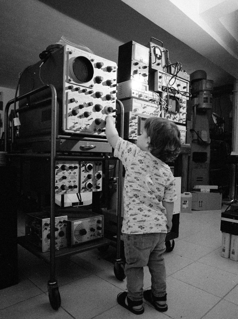
ON THE COVER: Nicholas Thermion Agnew (22 months old) getting an early start on a vintage Tektronix Type 545B and several other measurement instruments at the Agnew Analog Reference Instruments laboratory (https://www.agnewanalog.com), near Thessaloniki, Greece. The vintage instruments and machine tools in the facility are still in daily use and regularly calibrated. The photograph was shot on film by J. I. Agnew (managing director, ASME, IEEE, ASPE, AES) and developed in-house.
UPCOMING CONFERENCES & MEETINGS
The following event dates and delivery methods are subject to change. Visit the event URL provided for the latest information.
Jan 17-18, 2023 IUPAC/CITAC Workshop on Metrology, Quality and Conformity Assessment. Tel Aviv, Israel . This Event will be held in conjunction with Isranalytica 2023 Conference and Exhibition, as its satellite event. Leading researchers from the academia, industry, and government agencies in Israel and overseas will present their achievements and discuss exciting developments in different fields. The program will consist of several plenary lectures by prominent international scientists, oral presentations (in parallel sessions), featuring speakers from Israel and abroad and a large poster session. https://www. citac.cc/conferences-and-workshops/
Jan 22-25, 2023 ARFTG Microwave
Feb 20-23, 2023 Metrology Society of Australasia (MSA) Conference. Wellington, New Zealand. Metrology Society of Australasia conferences are a rare opportunity to demonstrate calibration, test and measurement products and services to a cross-section of measurement-focused scientists, engineers and technicians from Australia, New Zealand and beyond. https://www.metrology.asn.au/ msaconnected/
Feb 27-Mar 1, 2023 NCSLI Technical Exchange. Houston, TX. Enhance your skills in the calibration of measurement and test equipment with three days of on-site and hands-on measurement training. https://ncsli.org/
Measurement
Conference. Las Vegas, NV. Measurement techniques, approaches and considerations for frequencies from RF through THz, Measurement based modeling, VNA calibration and measurement uncertainties and other related topics are also covered. https://www.arftg.org/
Mar 7-10, 2023 21st International Metrology Congress (CIM). Lyon, France. The 21st International Metrology Congress (CIM) is the one event in Europe where metrology meets science, industry and quality infrastructure bodies! https://www.cim2023.com/
Web: www.thunderscientific.com Email: sales@thunderscientific.com Phone: 800.872.7728
Model 2900 FEATURES
• Traceable to SI
• Multi-point Touch LCD
• 0.5% of Reading RH Uncertainty
• High Flow Capability of 50 L/min
• Externally Driven Chamber Fan
• Fluid Jacketed Chamber Door
• Optional Window Chamber Door
• Ability to Operate Using External Computer
• Embedded ControLog® Automation Software
Use of the NVLAP symbol does not imply product certification, approval, or endorsement by NVLAP, NIST, or any agency of the U.S. Government.
Thunder’s calibration laboratory offers NVLAP accredited humidity calibration services which adheres to the guidelines of ISO/IEC 17025:2017 and ANSI/NCSL Z540-1-1994; Part 1. Ask for Guard Banding options.


• Based on NIST Proven “Two-Pressure” Principle
• HumiCalc® with Uncertainty Mathematical Engine
• Generate: RH, DP, FP, PPM, Multi-point Profiles
Model 3920 FEATURES
• Traceable to SI
• Multi-point Touch LCD
• Calculated Real-Time Uncertainty
• High Flow Capability of 10 L/min
• Diaphragm-sealed Control Valves
• Calculated Water Capacity/Usage
• VCR® Metal Gasket Face Seal Fittings
• Ability to Operate Using External Computer
• Embedded ControLog® Automation Software
• Based on NIST Proven “Two-Pressure” Principle


• HumiCalc® with Uncertainty Mathematical Engine
• Generate: RH, DP, FP, PPM, Multi-point Profiles
2 Oct • Nov • Dec 2022 Cal Lab: The International
CALENDAR
Humidity Generation and Calibration Equipment The Humidity Source ® Calibration Services Technical Support Sales & Service New Model 3920 CALIBRATION NVLAP Lab Code 200582-0
“Two-Pressure” Humidity Generation System
Journal of Metrology
Model 3920 Low Humidity Generation System
Model 2900
CalLab-Ad-2022.indd 1 11/16/2022 1:25:05 PM
PUBLISHER
MICHAEL L. SCHWARTZ
EDITOR
SITA P. SCHWARTZ
CAL LAB PO Box 111113 Aurora, CO 80042 TEL 303-317-6670 • FAX 303-317-5295 office@callabmag.com www.callabmag.com
E DITORIAL ADVISORS
CHRISTOPHER L.
GRACHANEN
NATIONAL INSTRUMENTS
MIKE SURACI
SURACI CONSULTING SERVICES LEAD ASSESSOR, ANAB MARTIN DE GROOT MARTINDEGROOT CONSULTANCY
JESSE MORSE MORSE METROLOGY
JERRY ELDRED TESCOM
Subscription fees for 1 year (4 issues) $50 for USA, $55 Mexico/Canada, $65 all other countries. Visit www.callabmag.com to subscribe.
Printed in the USA.
© Copyright 2022 CAL LAB. ISSN No. 1095-4791
EDITOR’S DESK
Say Goodbye
This Editor's Desk is dedicated to my mom.
By the time you read this, 2023 is the year you’ll be filling in on forms and checks. 2022 was a year for hangovers, real and metaphorical. Coming out of the pandemic, it was also a transitional year, learning to navigate online and hybrid training and events, changing jobs, or even careers! It was also a time to reconnect with family and colleagues. I hope you all got to do all that. If you haven’t already, there’s no time like the present!
For this issue, Henry Zumbrun follows up with Part 2 of his “Force Calibration Guidance for Beginners.” In this second installment, load cells are covered in detail, the role of digital indicators are examined, and a glossary of terms provided to wrap it up. Henry is prolific with his force and uncertainty articles. More can be found on our website by searching for Zumbrun, or by going to mhforce.com and clicking on Documentation Tools.
In anticipation of the upcoming 10th International Symposium of Temperature (ITS 10 ) and its one hundredth anniversary, we are including a paper from the last event, ITS9. “Effects of Impurities on the Freezing Plateau of the Triple Point of Water” is republished here with permissions. Observations presented in this paper are as relevant today as they were when first published in 2012.
Finally, we have the second part of Hening Huang’s “Practitioner’s Perspective on the GUM Revision” where he provides a couple of alternative approaches using four examples, as well as resolutions to the Ballico paradox.
On a personal note: Despite a collective relief to “get back to normal,” respiratory diseases continue to impact many families this season. Please take care of one another by getting whatever vaccinations are available to you. Some individuals are more vulnerable than others and no amount of vaccinations, they get for themselves, will keep them safe.
To 2022, I say goodbye and good riddance — may 2023 be a better year for all of us.
Happy Measuring, Sita Schwartz Editor
Cal Lab: The International Journal of Metrology
3 Oct • Nov • Dec
2022
CALENDAR
Mar 27-31, 2023 23rd International Conference on Radionuclide Metrology and its Applications (ICRM)
This scientific event will continue the tradition of the previous ICRM conferences in order to present new developments and enhance the international collaboration in the field of radionuclide metrology. https://icrm2023. nipne.ro/
Apr 3-7, 2023 10th International Temperature Symposia (ITS10). Anaheim, CA. The International Temperature Symposia have taken place approximately every 10 years since 1919. These Symposia provide opportunities for the presentation and publication of work related to the measurement and control of temperature, with topics ranging from fundamental research on temperature scales to practical measurement or control solutions in a variety of fields.https://its10.msc-conf.com/
Apr 4-7, 20223 MSC Training Symposium. Anaheim, CA. The 2023 MSC Symposium will offer many exceptional measurement courses and technical sessions presented by industry subject matter experts. The NIST Seminars,
ASQ Training, Tutorial Workshops and Technical Sessions along with Hands On practical application courses, will broaden one’s knowledge and application skills in a wide array of measurement disciplines. https://annualconf. msc-conf.com/
Apr 16-19, 2023 A2LA Annual Conference. Tucson, AZ. Conference attendees include professionals working in a wide variety of roles and all levels of experience. Presenters come from all over the world. Like many of the conference attendees, they return each year for the unique opportunity to connect with peers and experience the exceptional hospitality from A2LA’s staff. https://a2la. org/annual_conference/
Apr 19-20, 2023 Metromeet (Industrial Dimensional Metrology) . Bilbao, Spain. METROMEET is a unique event and the most important annual conference in the sector of Industrial Dimensional Metrology. https:// metromeet.org
Apr 24-28, 2023 International Conference on Smart

4 Oct • Nov • Dec 2022
Cal Lab: The International Journal of Metrology
Grid Technology (SMAGRIMET). Dubrovnik, Croatia. The Conference program will feature a comprehensive and high-quality technical program, including expert keynotes, several tutorials, and workshops. https:// smagrimet.org/2023/

Apr 24-26, 2023 International Conference of Weighing (ICW). Hamburg, Germany. https://www. weighingconference.com/
May 8-11, 2023 Sensor and Measurement Science International (SMSI). Nürnberg, Germany. The Sensor and Measurement Science International (SMSI) brings scientists and researchers from all concerned scientific fields together to secure the success of these ideas in the future. https://www.smsi-conference.com/
May 9-11, 2023 SENSOR+TEST . Nürnberg, Germany. SENSOR+TEST is the leading forum for sensors, measuring and testing technologies worldwide. https:// www.sensor-test.de/
May 15-18, 2023 CCM & IMEKO International Conference on Pressure and Vacuum Metrology Washington, DC. https:// www.nist.gov/news-events/ events/2023/05/2023-ccm-imeko-international-conferencepressure-and-vacuum-metrology
May 22-25, 2023 International Instrumentation and Measurement Technology Conference (I2MTC). Kuala Lumpur, Malaysia. The Conference focuses on all aspects of instrumentation and measurement science and technology research development and applications. https://i2mtc2023.ieee-ims.org/
May 29-31, 2023 IEEE International Workshop on Metrology for Living Environment (MetroLivEnv). Milan, Italy. IEEE International Workshop on Metrology for Living Environment (MetroLivEnv) aims to discuss the contributions of the metrology for the life cycle of the living environment and the new opportunities offered by the living environment for the development of new measurement methods and apparatus. https://www. metrolivenv.org
Integrated enterprise-level metrology software
When quality and accuracy are mission critical
moxpage.com 800-961-9410
5 Oct • Nov • Dec 2022
Lab: The International Journal of Metrology
Cal
CALENDAR
CALENDAR
SEMINARS & WEBINARS: Dimensional
Jan 10-11, 2023 “Hands-On” Precision Gage Calibration & Repair Training. Virtual. IICT Enterprises. This 2-day training offers specialized training in calibration and repair for the individual who has some knowledge of basic Metrology. Approximately 75% of the workshop involves “Hands-on” calibration, repair and adjustments of micrometers, calipers, indicators height gages, etc. https:// www.calibrationtraining.com/
Jan 24-26, 2023 Dimensional Gage Calibration. Aurora, IL. Mitutoyo. The course combines modern calibration and quality management ideas with best practices and “how-to” calibration methods for common calibrations. https://www. mitutoyo.com/training-education/classroom/
Jan 26-27, 2023 “Hands-On” Precision Gage Calibration & Repair Training. Bloomington, MN. IICT Enterprises. This 2-day training offers specialized training in calibration and repair for the individual who has some knowledge of basic Metrology. Approximately 75% of the workshop involves “Hands-on” calibration, repair and adjustments of micrometers, calipers, indicators height gages, etc. https:// www.calibrationtraining.com/
Feb 7-8, 2023 “Hands-On” Precision Gage Calibration & Repair Training. Schaumburg, IL.IICT Enterprises. This 2-day training offers specialized training in calibration and repair for the individual who has some knowledge of basic Metrology. Approximately 75% of the workshop involves “Hands-on” calibration, repair and adjustments of micrometers, calipers, indicators height gages, etc. https:// www.calibrationtraining.com/
Feb 9-10, 2023 “Hands-On” Precision Gage Calibration & Repair Training. Madison, WI. IICT Enterprises. This 2-day training offers specialized training in calibration and repair for the individual who has some knowledge of basic Metrology. Approximately 75% of the workshop involves “Hands-on” calibration, repair and adjustments of micrometers, calipers, indicators height gages, etc. https:// www.calibrationtraining.com/
Feb 14-16, 2023 Dimensional Gage Calibration. Aurora, IL. Mitutoyo. The course combines modern calibration and quality management ideas with best practices and “how-to” calibration methods for common calibrations. https://www. mitutoyo.com/training-education/classroom/
Feb 21-22, 2023 “Hands-On” Precision Gage Calibration & Repair Training. Virtual. IICT Enterprises. This 2-day training offers specialized training in calibration and repair for the individual who has some knowledge of basic Metrology. Approximately 75% of the workshop
involves “Hands-on” calibration, repair and adjustments of micrometers, calipers, indicators height gages, etc. https:// www.calibrationtraining.com/
Mar 14-15, 2023 “Hands-On” Precision Gage Calibration & Repair Training. Virtual. IICT Enterprises. This 2-day training offers specialized training in calibration and repair for the individual who has some knowledge of basic Metrology. Approximately 75% of the workshop involves “Hands-on” calibration, repair and adjustments of micrometers, calipers, indicators height gages, etc. https:// www.calibrationtraining.com/
Mar 21-22, 2023 “Hands-On” Precision Gage Calibration & Repair Training. Bloomington, MN. IICT Enterprises. This 2-day training offers specialized training in calibration and repair for the individual who has some knowledge of basic Metrology. Approximately 75% of the workshop involves “Hands-on” calibration, repair and adjustments of micrometers, calipers, indicators height gages, etc. https:// www.calibrationtraining.com/
Mar 21-23, 2023 Dimensional Gage Calibration. Aurora, IL. Mitutoyo. The course combines modern calibration and quality management ideas with best practices and “how-to” calibration methods for common calibrations. https://www. mitutoyo.com/training-education/classroom/
Apr 18-20, 2023 Dimensional Gage Calibration. Aurora, IL. Mitutoyo. The course combines modern calibration and quality management ideas with best practices and “how-to” calibration methods for common calibrations. https://www. mitutoyo.com/training-education/classroom/
May 1-2, 2024 Dimensional Measurement. Port Melbourne, VIC. National Measurement Institute, Australia. This two-day course (9 am to 5 pm) presents a comprehensive overview of the fundamental principles in dimensional metrology and geometric dimensioning and tolerancing. https://shop.measurement.gov.au/collections/physicalmetrology-training
May 16-18, 2023 Dimensional Gage Calibration. Aurora, IL. Mitutoyo. The course combines modern calibration and quality management ideas with best practices and “how-to” calibration methods for common calibrations. https://www. mitutoyo.com/training-education/classroom/
SEMINARS & WEBINARS: Education
Feb 23, 2023 Metric System Estimation. Adobe Connect Pro. NIST. This 1.5 hour session presents The Metric Estimation Game, a fun hands-on activity that helps middle students become familiar with SI measurements by practicing estimation skills. https://www.nist.gov/pml/owm/training
6 Oct • Nov • Dec 2022 Cal
Lab: The International Journal of Metrology

SEMINARS & WEBINARS: Electrical


Mar 6-9, 2023 Basic Hands-On Metrology. Everett, WA. Fluke Calibration. This Metrology 101 basic metrology training course introduces the student to basic measurement concepts, basic electronics related to measurement instruments and math used in calibration. https:// us.flukecal.com/training
Apr 3-6, 2023 Advanced Hands-On Metrology. Everett, WA. Fluke Calibration. This course introduces the student to advanced measurement concepts and math used in standards laboratories. https://us.flukecal.com/training
Apr 26-27, 2023 Electrical Measurement. Online. National Measurement Institute, Australia. This two day (9am5pm) course covers essential knowledge of the theory and practice of electrical measurement using digital multimeters and calibrators; special attention is given to important practical issues such as grounding, interference and thermal effects. https://shop.measurement.gov.au/ collections/physical-metrology-training
Jun 12-15, 2023 Basic Hands-On Metrology. Everett, WA. Fluke Calibration. This Metrology 101 basic metrology training course introduces the student to basic measurement concepts, basic electronics related to measurement instruments and math used in calibration. https://us.flukecal.com/training
SEMINARS & WEBINARS: Flow
Mar 29-30, 2023 Calibration of Liquid Hydrocarbon Flow Meters. Online. National Measurement Institute, Australia. This two-day course provides training on the calibration of liquid-hydrocarbon LPG and petroleum flow meters. It is aimed at manufacturers, technicians and laboratory managers involved in the calibration and use of flowmeters. https://shop.measurement.gov.au/collections/physicalmetrology-training

Apr 11-14, 2023 Gas Flow Calibration Using molbloc/ molbox. Phoenix, AZ. Fluke Calibration. Gas Flow Calibration Using molbloc/molbox is a four day training course in the operation and maintenance of a Fluke
8 Oct • Nov • Dec 2022 Cal Lab: The International Journal of Metrology CALENDAR ISO/IEC 17025:2017 CALIBRATION CERT #2746.01 Your Source for High Voltage Calibration. High Voltage Dividers & Probes HV CALIBRATION LAB CAPABILITIES: • UP TO 450kV PEAK 60Hz • UP TO 400kV DC • UP TO 400kV 1.2x50 μ s LIGHTNING IMPULSE DESIGN, MANUFACTURE, TEST & CALIBRATE: • HV VOLTAGE DIVIDERS • HV PROBES • HV RELAYS • HV AC & DC HIPOTS • HV DIGITAL VOLTMETERS • HV CONTACTORS • HV CIRCUIT BREAKERS • HV RESISTIVE LOADS • SPARK GAPS • FIBER OPTIC SYSTEMS HV LAB CALIBRATION STANDARDS ISO/IEC 17025:2017 ACCREDITED ANSI/NCSLI Z540-1-1994 ACCREDITED ISO 9001:2015 QMS CERTIFIED N.I.S.T. TRACEABILITY N.R.C. TRACEABILITY H IGH V OLTAGE C ALIBRATION L AB ENGINEERING CORPORATION ROSS 540 Westchester Drive, Campbell, CA 95008 USA | Ph: 408-377-4621 info@rossengineeringcorp.com | www.rossengineeringcorp.com ISO 9001:2015 QMS CERTIFIED
Calibration molbloc/molbox system. https://us.flukecal. com/training
SEMINARS & WEBINARS: General
Jan 30-Feb 3, 2023 Fundamentals of Metrology. Gaithersburg, MD. The 5-day Fundamentals of Metrology seminar is an intensive course that introduces participants to the concepts of measurement systems, units, good laboratory practices, data integrity, measurement uncertainty, measurement assurance, traceability, basic statistics and how they fit into a laboratory Quality Management System. https://www.nist.gov/pml/owm/ training
Feb 27-Mar 3, 2023 Fundamentals of Metrology. Gaithersburg, MD. The 5-day Fundamentals of Metrology seminar is an intensive course that introduces participants to the concepts of measurement systems, units, good laboratory practices, data integrity, measurement uncertainty, measurement assurance, traceability, basic statistics and how they fit into a laboratory Quality
Management System. https://www.nist.gov/pml/owm/ training
Mar 1, 2023 Calibration and Measurement Fundamentals. Online. National Measurement Institute, Australia. This course covers general metrological terms, definitions and explains practical concept applications involved in calibration and measurements. The course is recommended for technical officers and laboratory technicians working in all industry sectors who are involved in making measurements and calibration process. https://shop.measurement.gov.au/ collections/physical-metrology-training
SEMINARS & WEBINARS: Industry Standards
Jan 9-12, 2023 Understanding ISO/IEC 17025:2017 for Testing & Calibration Laboratories. Virtual. A2LA WorkPlace Training. This course is a comprehensive review of the philosophies and requirements of ISO/IEC 17025:2017. The participant will gain an understanding of conformity assessment using the risks and opportunitiesbased approach. https://www.a2lawpt.org/events
PURITY AND PRECISION
•
•
•
•
•
•
• Wireless Option
9 Oct • Nov • Dec 2022 Cal
Lab: The International Journal of Metrology CALENDAR
The
Gauge Visit ralstoninst.com/CL-SG or scan the QR code to find out more +1-440-564-1430 | (US/CA) 800-347-6575 ISO 9001:2015 Certified Made in the U.S.A. These digital
gauges maintain accuracy around vibrations,
hot
and other harsh processes common in the food & beverage, pharmaceutical
industries.
LC20 Diaphragm Pressure
sanitary
pulsations,
caustic rinses,
and biotech
± 0.1% full scale accuracy (ASME B40.100 Grade 4A/ ISO Class 0.1)
3-A certified sanitary Tri-Clamp® diaphragm seals
Clean or steam in place (CIP/SIP)
316L SS body and diaphragm
18-24 RA wetted surface finish
High temperature pipe sealant and tamper-proof inspection seal used on all threaded joints
CALENDAR
Jan 23-26, 2023. Auditing Your Laboratory to ISO/IEC 17025:2017. Virtual. A2LA WorkPlace Training. This ISO/IEC 17025 auditor training course will introduce participants to ISO/IEC 19011, the guideline for auditing management systems as applied to ISO/IEC 17025:2017. https://www.a2lawpt.org/events
Jan 24-25, 2023 Understanding ISO/IEC 17025 for Testing and Calibration Labs. Online. IAS. The objective of this course is to learn about ISO/IEC 17025 from one of its original authors. To learn its Principles and what it requires of laboratory staff. https://www.iasonline.org/training/
Jan 31-Feb 1, 2023 Measurement Confidence: Fundamentals. Live Online. ANAB. This Measurement Confidence course introduces the foundational concepts of measurement traceability, measurement assurance and measurement uncertainty as well as provides a detailed review of applicable requirements from ISO/IEC 17025 and ISO/IEC 17020. https://anab.ansi.org/training
Feb 1-2, 2023 Internal Auditing for All Standards. Online. IAS. The course includes easy-to-implement methods for risk-based thinking, continual improvement, and closing out findings through the analysis of root causes aimed at their elimination. https://www.iasonline.org/training/
Feb 6-9, 2023 Understanding ISO/IEC 17025:2017 for Testing & Calibration Laboratories. Virtual. A2LA WorkPlace Training. This course is a comprehensive review of the philosophies and requirements of ISO/IEC 17025:2017. The participant will gain an understanding of conformity assessment using the risks and opportunitiesbased approach. https://www.a2lawpt.org/events
Feb 7-8, 2023 Laboratories: Understanding the Requirements and Concepts of ISO/IEC 17025:2017 . Live Online. ANAB. This introductory course is specifically designed for those individuals who want to understand the requirements of ISO/IEC 17025:2017 and how those requirements apply to laboratories. https://anab.ansi.org/ training
Feb 7-9, 2023 Internal Auditing to ISO/IEC 17025:2017 (Non-Forensic) . Live Online. ANAB. ISO/IEC 17025 training course prepares the internal auditor to clearly understand technical issues relating to an audit. Attendees of Auditing to ISO/IEC 17025 training course will learn how to coordinate a quality management system audit to ISO/ IEC 17025:2017 and collect audit evidence and document observations. https://anab.ansi.org/training
Feb 13-16, 2023. Auditing Your Laboratory to ISO/IEC 17025:2017. Virtual. A2LA WorkPlace Training. This ISO/IEC 17025 auditor training course will introduce
participants to ISO/IEC 19011, the guideline for auditing management systems as applied to ISO/IEC 17025:2017. https://www.a2lawpt.org/events
Feb 22-23, 2023 Understanding ISO/IEC 17025 for Testing and Calibration Labs. Online. IAS. The objective of this course is to learn about ISO/IEC 17025 from one of its original authors. To learn its Principles and what it requires of laboratory staff. https://www.iasonline.org/training/
Mar 1-2, 2023 Understanding ISO/IEC 17025 for Testing and Calibration Labs. Online. IAS. The objective of this course is to learn about ISO/IEC 17025 from one of its original authors. To learn its Principles and what it requires of laboratory staff. https://www.iasonline.org/training/
Mar 14-15, 2023 Laboratories: Understanding the Requirements and Concepts of ISO/IEC 17025:2017. Live Online. ANAB. This introductory course is specifically designed for those individuals who want to understand the requirements of ISO/IEC 17025:2017 and how those requirements apply to laboratories. https://anab.ansi.org/ training
Mar 14-16, 2023 Internal Auditing to ISO/IEC 17025:2017 (Non-Forensic) . Live Online. ANAB. ISO/IEC 17025 training course prepares the internal auditor to clearly understand technical issues relating to an audit. Attendees of Auditing to ISO/IEC 17025 training course will learn how to coordinate a quality management system audit to ISO/ IEC 17025:2017 and collect audit evidence and document observations. https://anab.ansi.org/training
Mar 22-23, 2023 Internal Auditing for All Standards. Online. IAS. The course includes easy-to-implement methods for risk-based thinking, continual improvement, and closing out findings through the analysis of root causes aimed at their elimination. https://www.iasonline. org/training/
Apr 19-20, 2023 Measurement Confidence: Fundamentals. Live Online. ANAB. This Measurement Confidence course introduces the foundational concepts of measurement traceability, measurement assurance and measurement uncertainty as well as provides a detailed review of applicable requirements from ISO/IEC 17025 and ISO/IEC 17020. https://anab.ansi.org/training
May 16-17, 2023 Laboratories: Understanding the Requirements and Concepts of ISO/IEC 17025:2017. Live Online. ANAB. This introductory course is specifically designed for those individuals who want to understand the requirements of ISO/IEC 17025:2017 and how those requirements apply to laboratories. https://anab.ansi.org/ training
Cal Lab: The International Journal of Metrology
10 Oct • Nov • Dec 2022

Telephone: 650 802-8292 • Email: sales@gmw.com bartington.com US distributor: gmw.com • Coil diameters from 350mm to 2m • Orthogonality correction using PA1 • Active compensation using CU2 • Control software available HC2 HC16 HC1 HELMHOLTZ COIL SYSTEMS Range of Fluxgate Magnetometers Available
CALENDAR
May 16-18, 2023 Internal Auditing to ISO/IEC 17025:2017 (Non-Forensic). Live Online. ANAB. ISO/IEC 17025 training course prepares the internal auditor to clearly understand technical issues relating to an audit. Attendees of Auditing to ISO/IEC 17025 training course will learn how to coordinate a quality management system audit to ISO/IEC 17025:2017 and collect audit evidence and document observations, including techniques for effective questioning and listening. https://anab.ansi.org/training
June 21-22, 2023 Measurement Confidence: Fundamentals. Live Online. ANAB. This Measurement Confidence course introduces the foundational concepts of measurement traceability, measurement assurance and measurement uncertainty as well as provides a detailed review of applicable requirements from ISO/IEC 17025 and ISO/IEC 17020. https://anab.ansi.org/training
SEMINARS & WEBINARS: Mass
Feb 6-17, 2023 Mass Metrology Seminar. Gaithersburg, MD. The Mass Metrology Seminar is a two-week, “handson” seminar. It incorporates approximately 30 percent lectures and 70 percent demonstrations and laboratory work in which the participant performs measurements by applying procedures and equations discussed in the classroom. https://www.nist.gov/pml/owm/training
Apr 10-21, 2023 Mass Metrology Seminar. Gaithersburg, MD. The Mass Metrology Seminar is a two-week, “handson” seminar. It incorporates approximately 30 percent lectures and 70 percent demonstrations and laboratory work in which the participant performs measurements by applying procedures and equations discussed in the classroom. https://www.nist.gov/pml/owm/training
Jul 17-27, 2023 Advanced Mass Seminar. Gaithersburg, MD. NIST. The 9-day, hands-on Advanced Mass calibration seminar focuses on the comprehension and application of the advanced mass dissemination procedures, the equations, and associated calculations. It includes the operation of the laboratory equipment, review of documentary references, reference standards, specifications, and tolerances relevant to the measurements. https://www.nist.gov/pml/owm/ training
SEMINARS & WEBINARS: Measurement Uncertainty
Jan 26-27, 2023 Measurement Confidence: Fundamentals and Practical Applications. Grapevine, TX. ANAB. This “hybrid” course combines the core content of two of our most popular curriculums: Measurement Confidence Fundamentals and Measurement Uncertainty Practical Applications, into a robust 2-day course that can only be
taught in-person. https://anab.ansi.org/training
Feb 14-16, 2023 Measurement Uncertainty: Practical Applications. Live Online. ANAB. This course reviews the basic concepts and accreditation requirements associated with measurement traceability, measurement assurance, and measurement uncertainty as well as their interrelationships. https://anab.ansi.org/training
Mar 6-7, 2023 Introduction to Measurement Uncertainty. Virtual. A2LA WorkPlace Training. This course is a suitable introduction for both calibration and testing laboratory participants, focusing on the concepts and mathematics of the measurement uncertainty evaluation process. https://www.a2lawpt.org/events
Mar 15-16, 2023 Uncertainty of Measurement for Labs. Online. IAS. Evaluation and Estimation of Uncertainties of Measurement. Introduction to metrology principles, examples and practical exercises. https://www.iasonline. org/training/
Mar 22-23, 2023 Uncertainty of Measurement for Labs. Online. IAS. Evaluation and Estimation of Uncertainties of Measurement. Introduction to metrology principles, examples and practical exercises. https://www.iasonline. org/training/
Apr 25-27, 2023 Measurement Uncertainty: Practical Applications. Live Online. ANAB. This course reviews the basic concepts and accreditation requirements associated with measurement traceability, measurement assurance, and measurement uncertainty as well as their interrelationships. https://anab.ansi.org/training
SEMINARS & WEBINARS: Pressure
Jan 30-Feb 3, 2023 Principles of Pressure Calibration Web-Based Training. Fluke Calibration. This is a short form of the regular five-day in-person Principles of Pressure Calibration class. It is modified to be an instructor-led online class and without the hands-on exercises. It is structured for two hours per day for one week. https://us.flukecal.com/training
Mar 27-31, 2023 Principles of Pressure Calibration. Phoenix, AZ. Fluke Calibration. A five-day training course on the principles and practices of pressure calibration using digital pressure calibrators and piston gauges (pressure balances). https://us.flukecal.com/training
Apr 24-28, 2023 Advanced Piston Gauge Metrology. Phoenix, AZ. Fluke Calibration. Focus is on the theory, use and calibration of piston gauges and dead weight testers. https://us.flukecal.com/training
Cal Lab: The International Journal of Metrology
•
12 Oct
Nov • Dec 2022
May 8-12, 2023 Principles of Pressure Calibration WebBased Training. Fluke Calibration. This is a short form of the regular five-day in-person Principles of Pressure Calibration class. It is modified to be an instructor-led online class and without the hands-on exercises. It is structured for two hours per day for one week. https:// us.flukecal.com/training
Jun 7-8, 2023 Pressure Measurement. Port Melbourne, VIC. National Measurement Institute, Australia. This two-day course (9 am to 5 pm each day) covers essential knowledge of the calibration and use of a wide range of pressure measuring instruments, their principles of operation and potential sources of error—it incorporates extensive handson practical exercises. https://shop.measurement.gov.au/ collections/physical-metrology-training
SEMINARS & WEBINARS: Software
Feb 6-10, 2023 MET/TEAM® Basic Web-Based Training Fluke Calibration. This web-based course presents an overview of how to use MET/TEAM® Test Equipment and Asset Management Software in an Internet browser to develop your asset management system. https:// us.flukecal.com/training
Feb 27-Mar 3, 2023 MET/CAL® Procedure Development Web-Based Training. Fluke Calibration. Learn to create procedures with the latest version of MET/CAL, without leaving your office. This web seminar is offered to MET/ CAL users who need assistance writing procedures but have a limited travel budget. https://us.flukecal.com/ training


Mar 20-24, 2023 Basic MET/CAL® Procedure Writing. Everett, WA. Fluke Calibration. In this five-day Basic MET/CAL ® Procedure Writing course, you will learn to configure MET/CAL ® software to create, edit, and maintain calibration solutions, projects and procedures. https://us.flukecal.com/training
Apr 17-21, 2023 MET/TEAM ® Asset Management. Everett, WA. Fluke Calibration. This five-day course presents a comprehensive overview of how to use MET/ TEAM® Test Equipment and Asset Management Software in an Internet browser to develop your asset management system. https://us.flukecal.com/training
May 8-12, 2023 Advanced MET/CAL® Procedure Writing. Everett, WA. Fluke Calibration. A five-day procedure writing course for advanced users of MET/CAL ®


13 Oct • Nov • Dec 2022 Cal Lab: The International Journal of Metrology CALENDAR SEE WWW OHM-LABS COM FOR DETAILS Model Resistance TCR / VCR 106 1 M < 1 / < 0.1 107 10 M < 3 / < 0.1 108 100 M < 10 / < 0.1 109 1 G < 15 / < 0.1 110 10 G < 20 / < 0.1 111 100 G < 30 / < 0.1 112 1 T < 50 / < 0.1 113 10 T < 300 / < 0.1 HIG H RESISTANCE STANDARDS 611 E. CARSON ST PITTSBURGH PA 15203 TEL 412-431-0640 FAX 412-431-0649 WWW OHM-LABS COM FULLY GUARDED CONSTRUCTION TYPE N, BPO OR BNC CONNECTORS OR TRIAX FOR LOW CURRENT CALIBRATION VERY LOW TCR & VCR STABLE OVER TIME INTERNAL TEMPERATURE SENSOR ISO 17025 ACCREDITED CALIBRATION
CALENDAR
calibrations software. https://us.flukecal.com/training
May 9-11, 2023 VNA Tools Training Course. BerneWabern, Switzerland. Federal Institute of Metrology METAS. VNA Tools is free software developed by METAS for measurements with the Vector Network Analyzer (VNA). The software facilitates the tasks of evaluating measurement uncertainty in compliance with the ISO-GUM and vindicating metrological traceability. The software is available for download at www.metas.ch/vnatools. The three day course provides a practical and hands-on lesson with this superior and versatile software. https://www. metas.ch/metas/en/home/dl/kurse---seminare.html
May 15-19, 2023 MET/TEAM® Basic Web-Based Training. Fluke Calibration. This web-based course presents an overview of how to use MET/TEAM® Test Equipment and Asset Management Software in an Internet browser to develop your asset management system. https://us.flukecal. com/training
Jun 5-9, 2023 MET/CAL ® Procedure Development Web-Based Training. Fluke Calibration. Learn to create procedures with the latest version of MET/CAL, without leaving your office. This web seminar is offered to MET/ CAL users who need assistance writing procedures but have a limited travel budget. https://us.flukecal.com/ training
SEMINARS & WEBINARS: Temperature & Humidity
Mar 15, 2023 Humidity Measurement. Online (TrainerDelivered). National Measurement Institute (NMI), Australia. This one-day course provides information about the main concepts and practical techniques involved in measuring humidity in air and explains how to make such measurements accurately and consistently.https:// shop.measurement.gov.au/collections/physical-metrologytraining
Mar 20-22, 2023 Practical Temperature Calibration. American Fork, UT. Fluke Calibration. A three-day course loaded with valuable principles and hands-on training designed to help calibration technicians and engineers get a solid base of temperature calibration fundamentals. https:// us.flukecal.com/training
Mar 23-24, 2023 Infrared Calibration. American Fork UT. Fluke Calibration. A two-day course with plenty of hands on experience in infrared temperature metrology. This course is for calibration technicians, engineers, metrologists, and technical experts who are beginning or sustaining an infrared temperature calibration program. https://us.flukecal.com/training
SEMINARS & WEBINARS: Time & Frequency
Apr 19-20, 2023 Time and Frequency Measurement. Lindfield, NSW. National Measurement Institute, Australia. This two-day course covers the broad range of equipment and techniques used to measure time and frequency and to calibrate time and frequency instruments. https://shop. measurement.gov.au/collections/physical-metrologytraining
SEMINARS & WEBINARS: Vibration
Feb 28-Mar 2, 2023 Fundamentals of Random Vibration and Shock Testing . San Diego, CA. This three-day Training in Fundamentals of Random Vibration and Shock Testing covers all the information required to plan, perform, and interpret the results of all types of dynamic testing. Some of the additional areas covered are fixture design, field data measurement and interpretation, evolution of test standards and HALT/HASS processes. https://equipment-reliability.com/open-courses/
SEMINARS & WEBINARS: Volume
Mar 6-10, 2023 Volume Metrology Seminar. Gaithersburg, MD. NIST. The 5-day OWM Volume Metrology Seminar is designed to enable metrologists to apply fundamental measurement concepts to volume calibrations. A large percentage of time is spent on hands-on measurements, applying procedures and equations discussed in the classroom. https://www.nist.gov/pml/weights-andmeasures/training
SEMINARS & WEBINARS: Weight
Mar 9-10, 2023 Calibration of Weights and Balances . Online (Webex). National Measurement Institute (NMI), Australia. This course covers the theory and practice of the calibration of weights and balances. It incorporates hands-on practical exercises to demonstrate adjustment features and the effects of static, magnetism, vibration and draughts on balance performance. https://shop. measurement.gov.au/collections/physical-metrologytraining
Visit www.callabmag.com for upcoming metrology events & webinars!
Cal Lab: The International Journal of Metrology
14
•
•
Oct
Nov
Dec 2022
Human- and Machine-Readable Key Comparison Reports Using the PDF/A-3 Format

The BIPM is pleased to announce the publication of the first key comparison report embedding machinereadable (XML and JSON) versions of the document. Use of the PDF/A-3 standard in this way was originally suggested by METAS (Switzerland) in the context of Digital Calibration Certificates (DCC) [https://doi.org/10.1016/j. measen.2021.100282].
The recent update of the BIPM.RI(II)-K1.Ce139 comparison – using the BIPM’s International Reference System (SIR) for
radionuclide metrology – provided an opportunity to introduce this approach for the first time in reporting a key comparison.
In the context of international key comparisons, the PDF/A-3 format offers the possibility for machines to automatically retrieve key comparison data and the rich metadata associated with it. Key comparison metadata include administrative and technical details of the corresponding measurements, and in the digital world they provide a valuable means of identifying the individual results, and enable advanced data analyses that are not feasible based on a document designed to be read only by humans.
Pending the development of a digitalized KCDB, the adoption of the PDF/A-3 format for comparison reports is a first step towards achieving the FAIR (Findable, Accessible, Interoperable, Reusable) principles.
Source: https://www.bipm.org/en/-/2022-09-30.
Permission: This story is reproduced with permission of the BIPM, which retains full internationally protected copyright (© BIPM – Reproduced with permission).
MULTIPRODUCT CALIBRATORS & PRECISION MULTIMETERS IN STOCK


15 Oct • Nov • Dec 2022 Cal Lab: The
Journal of Metrology
International
A wide range of Multiproduct Calibrators: 80ppm, 50ppm, 25ppm, 15ppm, 8ppm Exceptional workload coverage at an a ordable price point, and... Three Year Warranty. 8.5 Digit DMMs: Wider Ranges, AC/DC Current to 30A, 4ppm and 9ppm Available. ADVANCED METROLOGY SYSTEMS
INDUSTRY AND RESEARCH NEWS
INDUSTRY AND RESEARCH NEWS
To Break New Ground With Frequency Combs, a NIST Innovation Plays With the Beat
NIST News, October 24, 2022 — An improvement to a Nobel Prize-winning technology called a frequency comb enables it to measure light pulse arrival times with greater sensitivity than was previously possible — potentially improving measurements of distance along with applications such as precision timing and atmospheric sensing.
The innovation, created by scientists at the National Institute of Standards and Technology (NIST), represents a new way of using frequency comb technology, which the scientists have termed a “time programmable frequency comb.” Up until now, frequency comb lasers needed to create light pulses with metronomic regularity to achieve their effects, but the NIST team has shown that manipulating the timing of the pulses can help frequency combs make accurate measurements under a broader set of conditions than has been possible.
“We’ve essentially broken this rule of frequency combs that demands they use a fixed pulse spacing for precision operation,” said Laura Sinclair, a physicist at NIST’s Boulder campus and one of the paper’s authors. “By changing how we control frequency combs, we have gotten rid of the trade-offs we had to make, so now we can get high-precision results even if our system only has a little light to work with.”
The team’s work is described in the journal Nature [DOI: 10.1038/s41586-022-05225-8].
Often described as a ruler for light, a frequency comb is a type of laser whose light consists of many well-defined frequencies that can be measured accurately. Looking at the laser’s spectrum on a display, each frequency would stand out like one tooth of a comb, giving the technology its name. After earning NIST’s Jan Hall a portion of the 2005 Nobel Prize in Physics, frequency combs have found use in a number of applications ranging from precision timekeeping to finding Earth-like planets to greenhouse gas detection.
Despite their many current uses, frequency combs do possess limitations. The team’s paper is an attempt to address some of the limitations that arise when using frequency combs to make precise measurements outside the laboratory in more challenging situations, where signals can be very weak.

Since shortly after their invention, frequency combs have enabled highly accurate measurements of distance. In part, this accuracy stems from the broad array of frequencies of light the combs use. Radar, which uses radio waves to determine distance, is accurate to anywhere from centimeters to many meters depending on the signal’s pulse width. The optical pulses from a frequency comb are far shorter than radio, potentially allowing measurements accurate to nanometers (nm), or billionths of a meter — even when the detector is many kilometers from the target. Use of frequency comb techniques could eventually enable precise formation flying of satellites for coordinated sensing of Earth or space, improving GPS, and supporting other ultra-precise navigation and timing applications.
Distance measurement using frequency combs requires two combs whose lasers’ pulse timing is tightly coordinated. The pulses from one comb laser are bounced off a faraway object, just as radar uses radio waves, and the second comb, slightly offset in repetition period, measures their return timing with great accuracy.
The limitation that comes with this great accuracy relates to the amount of light that the detector needs to receive. By nature of its design, the detector can only register photons from the ranging laser that arrive at the same time as pulses from the second comb’s laser. Up to now, due to the slight offset in repetition period, there was a relatively lengthy period of “dead time” between these pulse overlaps, and any photons that arrived between the overlaps were lost information, useless to the measurement effort. This made some targets hard to see.
Physicists have a term for their aspirations in this case: They want to make measurements at the “quantum limit,” meaning they can take account of every available photon that carries useful information. More photons detected means greater ability to spot fast changes in distance to a target, a goal in other frequency comb applications. But for all its accomplishments to date, frequency comb technology has operated far from that quantum limit.
“Frequency combs are commonly used to measure physical quantities such as distance and time with extreme accuracy, but most measurement techniques waste the great majority of the light, 99.99% or more,” Sinclair said. “We have instead shown that by using this different control method, you can get rid of that waste. This can mean an increase in measurement speed, in precision, or it allows using a much smaller system.”
The team’s innovation involves the ability to control the timing of the second comb’s pulses. Advances in digital technology permit the second comb to “lock on” to the returning signals, eliminating the dead time created by the previous sampling approach. This occurs despite the fact that the controller must find a “needle in a haystack” — the pulses are comparatively brief, lasting only 0.01% as long the dead time between them. After an initial acquisition, if the target moves, the digital controller can adjust the time output such that the second comb’s pulses speed up or slow
16 Oct • Nov • Dec 2022 Cal Lab:
The International Journal of Metrology
Optical frequency combs allow scientists to measure light — and our world — with great precision and accuracy. This device has led to innovations that scientists never imagined when it was created.
Credit: J. Wang/NIST
800-828-1470 | TRANSCAT.COM ENSURE ACCURACY | MITIGATE RISK | REDUCE COST Trust your instruments are performing accurately by using Transcat, North America’s leading provider of quality accredited calibration services. Contact Us for a FREE Calibration Quote Today! Make Sure Your Instrument is
INDUSTRY AND RESEARCH NEWS
down. This allows the pulses to realign, so that the second comb’s pulses always overlap with those returning from the target. This adjusted time output is exactly twice the distance to the target, and it is returned with the pinpoint precision characteristic of frequency combs.
The upshot of this time-programmable frequency comb, as the team calls it, is a detection method that makes the best use of the available photons — and eliminates dead time.
“We found we can measure the range to a target fast, even if we only have a weak signal coming back,” Sinclair said. “Since every returning photon is detected, we can measure the distance near the standard quantum limit in precision.”
Compared to standard dual-comb ranging, the team saw a 37-decibel reduction in required received power — in other words, only requiring around 0.02% of the photons needed previously.
The innovation could even enable future nanometer-level measurements of distant satellites, and the team is exploring how its time-programmable frequency comb could benefit other frequency comb sensing applications.
Source: https://www.nist.gov/news-events/news/2022/10/ break-new-ground-frequency-combs-nist-innovation-playsbeat
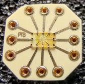
Resistance Measurements Using Graphene
PTBnews 3.2022 - Quantum Hall resistors made of graphene as primary impedance standards were optimized for AC voltage applications in a European metrology research project. They can now be operated with considerably less effort. This means that a larger number of metrology institutes and –beyond that – industrial calibration laboratories are now able to realize the units of resistance, capacitance and inductance.
Up to now, quantum Hall resistors made of semiconductor heterostructures have been used in electrical quantum metrology. In comparison, quantum Hall resistors made of graphene can be operated with considerably less technical effort. If the material quality is suitable and the charge carrier density is stable, these resistors allow resistance quantization to be realized at lower magnetic fields and at temperatures that are not so low.
Within the scope of an EMPIR project titled “Graphene Impedance Quantum Standard,” which is coordinated by PTB and involves 11 partners from Europe and Asia, graphene quantum Hall resistors were manufactured at PTB’s Clean Room Center using optimized procedures. Measurements performed at the BIPM (the International Bureau of
OKAY. SO, THIS IS THE “MEGA-RESOLUTION” OPTION?
18 Oct • Nov • Dec 2022
Cal Lab: The International Journal of Metrology
CAL-TOONS by Ted Green teddytoons@icloud.com
INDUSTRY AND RESEARCH NEWS
Weights and Measures) have confirmed the high quality of these devices: Their DC resistance is in agreement with the nominal quantized value to a few parts in a billion, even at a relatively high temperature of 4.2 K and a magnetic field of only 5 T. Comparison measurements carried out at the institutes involved in the project have demonstrated the temporal stability of the device properties and have shown that their high quality is hardly affected by long-distance transport. The main prerequisites for the future practical use of graphene-based quantum resistance standards are thus fulfilled.
The envisaged use of such standards in AC operation (i.e., for measuring impedance quantities) places additional requirements on the measuring instruments and the graphene
devices themselves. The devices manufactured at PTB were investigated in the laboratories of eight project partners using diverse methods. For this purpose, different types of impedance bridges were optimized during the project. PTB provided a Josephson impedance bridge which uses precise reference voltages generated by modern quantum voltage sources (based on the Josephson Effect). This leads to particularly high flexibility as regards the experimental parameters; it also allows automated measurement cycles to be used. In addition, the measuring system is more userfriendly. For impedance and frequency measurements, the accessible measuring ranges have been extended.
All in all, the project results were such that a quantumbased realization of the unit of capacitance, the farad, is now possible with a relative uncertainty of better than 10–7. This was summarized in the form of a good practice guide for the realization of the farad by means of graphene quantum standards (https://www.ptb.de/empir2019/giqs/home/). The new measurement capabilities will be made accessible to interested user groups within the scope of the Quantum Technology Competence Center of PTB.
Source: https://www.ptb.de/cms/en/presseaktuelles/ journals-magazines/ptb-news.html
19 Oct • Nov • Dec 2022
Cal Lab: The International Journal of Metrology
Graphene quantum Hall resistor developed and manufactured at PTB and electrically connected in its sample holder. Credit: PTB
Force Calibration Guidance for Beginners, Part 2
Henry Zumbrun Morehouse Instrument Company
Introduction
This two-part article was written to help anyone new to force. Even seasoned metrologists or technicians with years of experience may learn something new, or maybe this document can act as a refresher for those who are more advanced. In either case, the knowledge gained will ultimately help you become better.
In Part 1, we defined force calibration, its importance, and some devices used to measure force. We differentiated compression and tension in relation to force calibration, as well as defining what we mean by “calibration.” Since ISO/IEC 17025 requires a corrective value for measurement uncertainties on certificates of calibration, we covered the documentation to help define these values. And, we ended with the importance of measurement uncertainties and traceability.
In Part 2 of Force Calibration for Beginners, we cover load cells: terminology, types, and troubleshooting. We also explain what a digital indicator does and provide a glossary of terms often used in force calibration.
Load Cell Terminology
Non-Linearity, Non-Repeatability, Hysteresis, and Static Error Band are common load cell terminology typically found on a load cell specification sheet. There are several more terms regarding the characteristics and performance of load cells. However, I chose these four because they are the most common specifications found on certificates of calibration.
When broken out individually, these terms can help you select the suitable load cell for an application. Some of these terms may not be as important today as they were years ago because better meters are available that overcome inadequate specifications. One example is Non-Linearity. An indicator capable of multiple span points can significantly reduce the impact of a load cell’s non-linear behavior.
The meanings of these terms are described in detail below.
Non-Linearity: The quality of a function that expresses a relationship that is not one of direct proportion. For force measurements, Non-Linearity is defined as the algebraic difference between the output at a specific load and the corresponding point
Table 1. Load Cell Specification Sheet
20 Oct • Nov • Dec 2022 Cal Lab: The International Journal of Metrology
METROLOGY 101
METROLOGY
101
Non-Linearity is one of the specifications that would be particularly important if the indicating device or meter used with the load cell only has a two-point span, such as capturing values at zero and capacity or close to capacity. The specification gives the end-user an idea of the anticipated error or deviation from the best fit straight line. However, suppose the end-user has an indicator capable of multiple span points or one that can use coefficients from an ISO 376 or ASTM E74 type calibration. In that case, the non-linear behavior can be corrected, and the error significantly reduced.
Figure 1. Non-Linearity Expressed Graphically
on the straight line drawn between the outputs at minimum load and maximum load. It usually is expressed in units of % of full scale. It is usually calculated between 40-60 % of the full scale.
Non-Linearity Calculations Ignoring Ending Zero Though Running It Through the Formula
One way to calculate Non-Linearity is to use the slope formula or manually perform the calibration by using the load cell output at full scale minus zero and dividing it by force applied at full scale and 0. For example, a load cell reads 0 at 0 and 2.00010 mV/V at 1000 lbf. The formula would be (2.00010-0)/ (1000-0) = 0.002. This formula gives you the slope of the line assuming a straight-line relationship. Note: There are some manufacturers who take a less conservative approach and use higher order quadratic equations.
Force Applied (lbf) Run 1 Adjusted Non-Linearity Baseline Non-Linearity (%FS) Non-Linearity Line 0 0.00000 0 0.000 Slope= 0.0020001 50 0.10008 0.1000050 0.004 Intercept= 0 100 0.20001 0.2000100 0.000 200 0.40002 0.4000200 0.000 300 0.60001 0.6000300 0.001 Non-linearity = 0.004 400 0.80002 0.8000400 0.001 (%FS) 500 1.00005 1.0000500 0.000 600 1.20002 1.2000600 0.002 700 1.40003 1.4000700 0.002 800 1.60004 1.6000800 0.002 900 1.80006 1.8000900 0.001 1000 2.00010 2.0001000 0.000 0 0.00000 0
Table 2. Non-Linearity Baseline
Non-Linearity
Plot the Non-Linearity baseline as shown below using the formula of force applied * slope + Intercept or y = mx +b. If we look at the 50 lbf point, this becomes 50 * 0.0020001 + 0 = 0.100005. Thus at 50 lbf, the Non-Linearity baseline is 0.100005.
To find the Non-Linearity percentage, take the mV/V value at 50 lbf minus the calculated value and divide by the full-scale output multiplied by 100 to convert it to a percentage. Thus, the numbers become ((0.10008-0.100005)/2.00010) *100) = 0.004 %.
Calculations Reducing Ending Zero
Force Applied (lbf) Run 1 Adjusted Non-Linearity Baseline Non-Linearity (%FS)
Non-Linearity Line 0 =(E7*$K$7+$K$8) =ROUND(ABS(F7-G7)/$F$18*100,3) Slope= =(F18-F7)/(E18-E7) 50 0.10008 =(E8*$K$7+$K$8) =ROUND(ABS(F8-G8)/$F$18*100,3) Intercept= 0 100 0.20001 =(E9*$K$7+$K$8) =ROUND(ABS(F9-G9)/$F$18*100,3) 200 0.40002 =(E10*$K$7+$K$8) =ROUND(ABS(F10-G10)/$F$18*100,3) 300 0.60001 =(E11*$K$7+$K$8) =ROUND(ABS(F11-G11)/$F$18*100,3) Non-linearity= 400 0.800015 =(E12*$K$7+$K$8) =ROUND(ABS(F12-G12)/$F$18*100,3) (%FS) =MAX(H7:H19) 500 1.00005 =(E13*$K$7+$K$8) =ROUND(ABS(F13-G13)/$F$18*100,3) 600 1.200015 =(E14*$K$7+$K$8) =ROUND(ABS(F14-G14)/$F$18*100,3) 700 1.400025 =(E15*$K$7+$K$8) =ROUND(ABS(F15-G15)/$F$18*100,3) 800 1.60004 =(E16*$K$7+$K$8) =ROUND(ABS(F16-G16)/$F$18*100,3) 900 1.80006 =(E17*$K$7+$K$8) =ROUND(ABS(F17-G17)/$F$18*100,3) 1000 2.0001 =(E18*$K$7+$K$8) =ROUND(ABS(F18-G18)/$F$18*100,3) 0 =(E19*$K$7+$K$8)
Table 3. Non-Linearity Calculations (Starts with cell E)
Cal Lab: The International Journal of Metrology
21 Oct • Nov • Dec 2022
METROLOGY 101
At Morehouse, our calibration lab sampled several instruments and recorded the following differences (Table 4).
Load cells from five different manufacturers were sampled, and the results were recorded. The differences between the ascending and descending points varied from 0.007 % (shear web type cell) to 0.120 % on a column type cell. On average, the difference was approximately 0.06 %. Six of the seven tests were performed using deadweight primary standards, which is accurate within 0.0016 % of the applied force.
Figure 2. Hysteresis Example
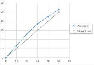
Hysteresis: The phenomenon in which the value of a physical property lags changes in the effect causing it. An example is when magnetic induction lags the magnetizing force. For force measurements, Hysteresis is often defined as the algebraic difference between output at a given load descending from the maximum load and output at the same load ascending from the minimum load.
Hysteresis is normally expressed in units of % full scale. It is normally calculated between 40 - 60 % of full scale. The graph above (Figure 2) shows a typical Hysteresis curve where the descending measurements have a slightly higher output than the ascending curve.
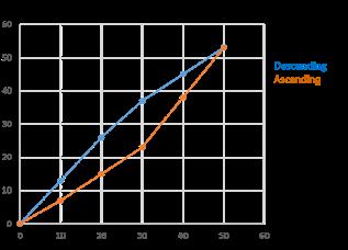
If the end-user uses the load cell to make descending measurements, then they may want to consider the effect of Hysteresis.
Errors from hysteresis can be high enough that if a load cell is used to make descending measurements, then it must be calibrated with a descending range. The difference in output on an ascending curve versus a descending curve can be significant. For example, an exceptionally good Morehouse 100K precision shear-web load cell had an output of -2.03040 on the ascending curve and -2.03126 on the descending curve. Using the ascending only curve would result in an additional error of 0.042 %.
Non-Repeatability: The maximum difference between output readings for repeated loadings under identical loading and environmental conditions. Normally this is expressed in units as a % of rated output (RO). Non-repeatability tells the user a lot about the performance of the load cell. It is important to note that non-repeatability does not tell the user about the load cell’s reproducibility or how it will perform under different loading conditions (randomizing the loading conditions). At Morehouse, we have observed numerous load cells with good non-repeatability specifications that do not perform well when the loading conditions are randomized or the load cell is rotated 120 degrees as required by ISO 376 and ASTM E74.
The calculation of non-repeatability is straightforward. First, compare each observed force point’s output and run a difference between those points. The formula would look something
22 Oct • Nov • Dec 2022 Cal Lab: The International Journal of Metrology
Table 4. Errors from Hysteresis Load Cell Manufacturer (names removed) 1 2 3 4 5 5 3 4 Ascending Output 50 % Force Point 1.49906 1.20891 -2.0304 24990 -5.18046 -2.49899 -2.0886 -2.15449 Descending Output 50 % Force Point 1.49947 1.21022 -2.03126 25020 -5.18265 -2.50103 -2.08846 -2.15579 Difference 0.027% 0.108% 0.42% 0.120% 0.042% 0.082% 0.007% 0.060% Non-Repeatability Calculations Run 1 Run 2 Run 3 4.0261 4.02576 4.02559 Difference b/w 1 & 2 (%FS) Difference b/w 1 & 3 (%FS) Difference b/w 2 & 3 (%FS) 0.0084 0.0127 0.0042 Non-Repeatability (%FS)= 0.013 Table 5. Non-Repeatability Numbers
METROLOGY 101
Non-Repeatability Calculations
=ABS(U4-V4)/AVERAGE($U$4:$W$4)*100 =ABS(U4-V4)/AVERAGE($U$4:$W$4)*100 =ABS(U4-V4)/AVERAGE($U$4:$W$4)*100
Non-Repeatability (%FS)= =MAX(U9:W9)
Table 6. Non-Repeatability Calculations
like this: Non repeatability = ABS(Run1-Run2)/ AVERAGE (Run1, Run2, Run3) *100. Do this for each combination or runs, and then take the maximum of the three calculations (Table 6).
Static Error Band: The band of maximum deviations of the ascending and descending calibration points from a best-fit line through zero output. It includes the effects of Non-Linearity, Hysteresis, and non-return to minimum load. It usually is expressed in units of % of full scale.
Because of what it captures, the Static error band might be the most exciting term. If the load cell is always used to make ascending and descending measurements, this term best describes the load cell’s actual error from the straight line drawn between the ascending and descending curves. Earlier, I noted that the end-user might want to consider the effects of Hysteresis unless they are using the load cell described above because a static
error band would be the better specification to use. The end-user could likely ignore Non-Linearity and Hysteresis and focus on static error band as well as non-repeatability.
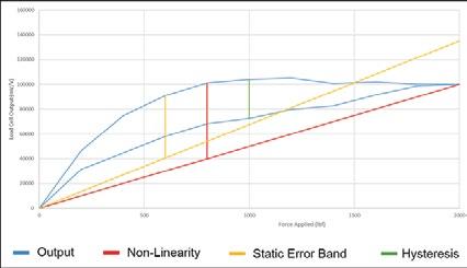
However, we find that many calibration laboratories primarily operate using ascending measurements, and on occasion, may have a request for descending data. When that is the case, the user may want to evaluate Non-Linearity and Hysteresis separately. When developing an uncertainty budget, use different budgets for each type of measurement, i.e., ascending and descending.
What needs to be avoided is a situation where a load cell is calibrated following a standard such as ASTM E74, or ISO 376, and additional uncertainty contributors for Non-Linearity and Hysteresis are added. ASTM E74 has a procedure and calculations that, when followed, uses a method of least squares to fit a polynomial function to the data points. The standard uses a specific term called the Lower Limit Factor (LLF), which is a statistical estimate of the error in forces computed from a force-measuring instrument’s calibration equation when the instrument is calibrated following the ASTM E74 practice.
To help differentiate between ASTM E74 and ISO 376, we published “An Introduction to the Differences Between the Two Most Recognized Force Standards.”1
https://www.callabmag.com/ an-introduction-to-the-differences-between-the-two-most-recognized-forcestandards/
Cal Lab: The International Journal of Metrology
23 Oct • Nov • Dec 2022
1
Figure 3. Static Error Band and Other Specifications Displayed Visually
Run 1 Run 2 Run 3 4.0261 4.02576 4.02559 Difference b/w 1 & 2 (%FS) Difference b/w 1 & 3 (%FS) Difference b/w 2 & 3 (%FS)
METROLOGY 101
Types of Load Cells
It is essential to understand the common types of load cells used in force measurement and choose your application’s suitable load cell.
The four types of load cells typically used in force measurement are bending beam, shear beam, miniature, and column. We are going to describe the common types we see used as reference and field standards below. Many other load cells are shown in more commercial applications, such as scales used at supermarket checkouts, weight sensing devices, weighing, and other scales.
S-Beam (S Type)
The S-beam is a bending beam load cell that is typically used in weighing applications under 50 lbf. These load cells work by placing a weight or generating a force on the load cell’s metal spring element, which causes elastic deformation. The strain gauges in the load cell measure the fractional change in length of the deformation. There are generally four strain gauges mounted in the load cell.
Figure 4. Types of Load Cells
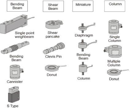
Shear Web
The shear web is a shear beam load cell that is ideal as a calibration reference standard up to 100,000 lbf. Shear web load cells are typically the most accurate when installed on a tapered base with an integral threaded rod installed.
Advantages:
Advantages:
• In general, linearity will be enhanced by minimizing the ratio of deflection at the rated load to the length of the sensing beam, thus minimizing the change in the shape of the element.
• Ideal for measuring small forces (under 10 lbf) when physical weights cannot be used.
• It is suited for scales or tension applications.
Disadvantages:
• The load cell is susceptible to off-axis loading.
• Compression output will be different if the load cell is loaded through the threads versus flat against each base.
• Typically, not the right choice for force applications requiring calibration to the following standards: ASTM E74, ASTM E4, ISO 376, and ISO 7500.
• Typically have very low creep and are not as sensitive to off-axis loading as the other load cells.
• Recommended choice for force applications from 100 lbf through 100,000 lbf.
Disadvantages:
• After 100,000 lbf, the cell’s weight makes it exceedingly difficult to use as a reference standard in the field. A 100,000 lbf shear web load cell weighs approximately 57 lbs, and a 200,000 lbf shear web load cell weighs over 120 lbs.
Watch this video2 showing a Morehouse load cell with only 0.0022 % off-axis error. If this load cell is used without a base or an integral top adapter, there may be significant errors associated with various loading conditions.
2 https://www.youtube.com/watch?v=MgTWK2hRHLs
24 Oct • Nov • Dec 2022 Cal Lab: The International Journal of Metrology
Button Load Cell
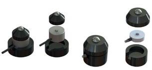
The button is a miniature load cell that is typically used when space is limited. It is a compact strain gauge-based sensor with a spherical radius that is often used in weighing applications.
Advantages:
• Suitable for applications where there is minimal room to perform a test.
Disadvantages:
• High sensitivity to off-axis or side loading. The load cell will produce high errors from any misalignment. For example, a 0.1 % misalignment can produce a significant cosine error. Some have errors anywhere from 1 % - 10 % of rated output.
• Does not repeat well in the rotation.
Advantages:
• Physical size and weight: It is common to have a 1,000,000 lbf column cell weigh less than 100 lbs.
Disadvantages:
• Reputation for inherent Non-Linearity. This deviation from linear behavior is commonly ascribed to the change in the column’s crosssectional area (due to Poisson’s ratio), which occurs with deformation under load.
• Sensitivity to off-center loading can be high.
• Larger creep characteristics than other load cells and often do not return to zero, as well as other load cells (ASTM Method A typically yields larger LLF).
• Different thread engagement can change the output.
• The design of this load cell requires a top adapter to be purchased with it. Varying the hardness of the top adapter will significantly change the output.
Multi-Column Load Cells
The multi-column is a column load cell that is good from 100,000 lbf through 1,000,000 plus lbf. The load is carried by four or more small columns in this design, each with its complement of strain gauges. The corresponding gauges from all the columns are connected in a series in the appropriate bridge arms.
Advantages:
• It can be more compact than single-column cells.
• Improved discrimination against the effects of off-axis load components.
• Typically have less creep and better zero returns than single-column cells.
• In many cases, a properly designed shear-web spring element can offer greater output, better linearity, lower hysteresis, and faster response.
Single-Column or High-Stress Load Cells
The single column is a column load cell that is good for general testing. The spring element is intended for axial loading and typically has a minimum of four strain gauges, with two in the longitudinal direction. Two are oriented transversely to sense the Poisson strain.
Disadvantages:
• The design of this load cell requires a top adapter to be purchased with it. Varying the hardness of the top adapter will change the output.
7. Lightweight 600 k (26 lb) Multi-Column Load Cell
Cal Lab: The International Journal of Metrology
25 Oct • Nov • Dec 2022
METROLOGY 101
Figure 5. Ultra-Precision Shear Web Load Cells
Figure 6. Button and Washer Load Cell Adapters
Figure
Load Cell Troubleshooting
Have you ever wasted hours troubleshooting a nonworking load cell to diagnose the problem? If you deal with load cells, you know how much of a time suck they can be when they are not working correctly. This section is designed to save you or your technicians valuable time by following an easy sevenstep troubleshooting guide. The time saved can be beneficial to get more calibrations done or spending more time getting the measurements correct by using the proper setups, adapters and understanding how to replicate how the end-user uses the device.
7 Step Process for Troubleshooting a Load Cell
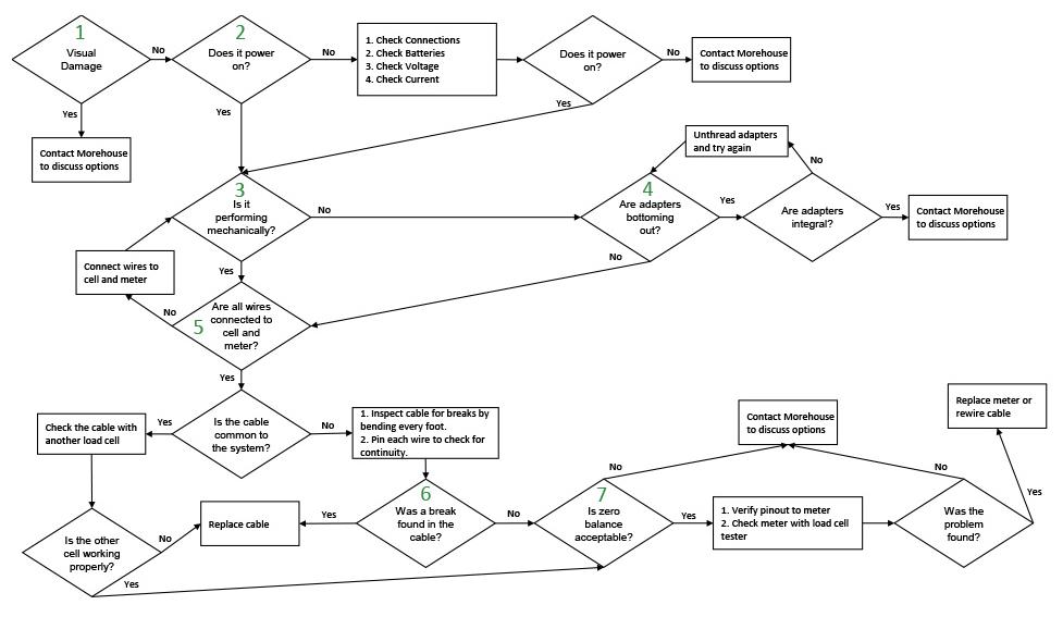
Morehouse technicians have seen many different load cell issues and have lots of experience identifying and fixing the problems. With this experience, we developed a “7 Step Process for Troubleshooting a Load Cell” to shorten our calibration lead time and provide better customer service.
This 7-step process outlined in Figure 8, and explained below, can help you save countless hours
trying to diagnose the problem with your load cell.
1. Visually inspect the load cell for noticeable damage.
2. Power on the system. Make sure all connections are made and verify batteries are installed and have enough voltage. Check the voltage and current on the power supply. If it still does not power on, then replace the meter. An inexpensive multimeter can be used for steps 2, 6, and 7.
26 Oct • Nov • Dec 2022 Cal Lab: The International Journal of Metrology
Figure 8. Load Cell Troubleshooting Process
Figure 9. Overloaded Load Cell
METROLOGY 101
3. If everything appears to be working, but the output does not make sense, check for mechanical issues. For example, some load cells have internal stops that may cause the output to plateau. Do not disassemble the load cell as it will void the manufacturer’s warranty and calibration. The best example of this error is that the load cell is very linear to 90 % of capacity. Then either the indicator stops reading, or the output becomes severely diminished. The data will show poor linearity when using 100 % of the range and incredibly good linearity when only using the data set to 90 % of the range.
4. Make sure any adapters threaded into the transducer are not bottoming out.3
5. Check and make sure the leads (all wires) are correctly connected to the load cell and meter. If the cable is common to the system, check another load cell and verify that the other cell is working correctly.
6. Inspect the cable for breaks. With everything hooked up, proceed to test the cable making a physical bend every foot. Pin each connection to check for continuity of the cable.
7. Use a load cell tester or another meter to check the load cell’s zero balance. If you do not have a load cell tester, you can check the bridge resistance with an ordinary multimeter. A typical Morehouse shear web load cell pins (A & D) and (B & C) should read about 350
3 Learn about adapters by reading https://www. callabmag.com/the-importance-of-adapters-in-force-measurement/.
OHMS ± 3.5. If one set reads high and another low (ex. (A & D) reads 349 and (B & C) reads 354), then there is a good chance that the load cell was overloaded.
Note: Different load cells use different strain gauges and have different resistance values. It is essential to check with the manufacturer on what they should read and the tolerance.
Diagnose with a Load Cell Tester
A load cell tester can be used to test for the following:
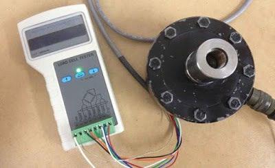
• Input and Output Resistance
• Resistance difference between sense and excitation leads.
• Signal Output
• Shield to Bridge
• Body to Bridge
• Shield to Body
• Linearity Watch this video4 showing how the load cell tester works.
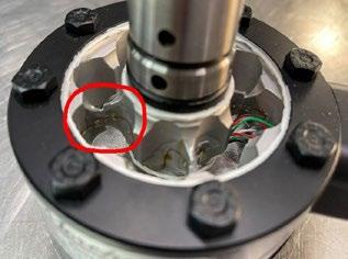
Overloaded Load Cell
It is important to note that if a load cell has been overloaded, mechanical damage has been done that is not repairable. Overloading causes permanent deformation within the flexural element and gauges, which destroys the carefully balanced processing. While it is possible to electrically re-zero a load cell following overload, it is not recommended because this does nothing to restore the affected performance parameters or the degradation to structural integrity.
4 https://www.youtube.com/ watch?v=zQNUpe2Bh5Y
Cal Lab: The International Journal of Metrology
27 Oct • Nov • Dec 2022
METROLOGY 101
Figure 10. Inside of an Overloaded Shear Web Load Cell Showing a Clear Break of the Web Element
Figure 11. Load Cell Tester
METROLOGY 101
Indicator Basics
When force is exerted on a load cell, the mechanical energy is converted into equivalent electrical signals. The load cell signal is converted to a visual or numeric value by a “digital indicator.” When there is no load on the cell, the two signal lines are at equal voltage. As a load is applied to the cell, the voltage on one signal line increases very slightly, while the voltage on the other signal line decreases very slightly.
The indicator reads the difference in voltage between the two signals that may be converted to engineering or force units. There are several types of indicators available, and they have different advantages and disadvantages. The decision for which indicator to use should be based on what meets your needs and has the best Non-Linearity and stability specifications.
Non-Linearity and Uncertainty Specification: The specification that most users look for in an indicator is the Non-Linearity. The better the NonLinearity is, the less the indicator will contribute to the system uncertainty.
Some indicators on the market may specify accuracies in terms of percentage of reading. Although these may include specifications such as 0.005 % of reading, they can cause negative impacts on the system’s uncertainty. The problem is that the resolution or number of digits may be such that the specification will not be maintained.
In other cases, the indicator may require adjustment at various span points to achieve NonLinearity between span points to meet the overall accuracy specifications claimed. The purpose of multi-spanning the range in an indicator is to divide the sensor output range into smaller segments and reduce Non-Linearity errors. However, accuracy claims can be questionable. Ensure the accuracy specification includes stability over time, repeatability, Non-Linearity, temperature characteristics, and consideration of the resolution or avoid this type of indicator.
Non-Linearity errors in a load system can be drastically reduced by:
• Employing the right calibration and measurement process
• Pairing a highly stable indicator to the load cell
• Having the system calibrated to highly accurate
standards such as Primary Deadweight Standards
• Using ASTM E74 or ISO 376 calibration coefficients to convert load cell output values into force units
Stability and Drift: This characteristic is often more difficult to quantify on non-high-end multimeters. Some indicators will specify thermal drift, longterm stability of zero, and some actual stability per range. The indicators often over $10,000 will fall into specifying drift at different intervals such as 90 days (about three months) and one year. Most indicators under $2,500 are not going to address 90 days or 1-year stability specifically. Stability can be monitored and maintained by a load cell simulator. However, a user can choose to live with the entire system drift of the load cell and indicator combined.
Resolution: If you use the indicator as a field system, a stable resolution of greater than 50,000 counts over the load cell’s output range will allow higher-order fits. It is also desirable for ASTM E74 calibrations because a higher-order fit will generally yield a Lower Limit Factor (LLF) and better Class AA and Class A loading ranges.
Number of Span Points: This assumes you require the actual display to read in engineering units and are not okay with 4.00001 mV/V representing 10,000.0 force units such as lbf or kN. However, any system’s downfall for direct reading is that it cannot be maintained. As the system drifts, so will the readings. Therefore, 10,000.0 today may equate to 10,000.9 in a year. Consequently, we highly recommend having the output read in mV/V and converting it via software or internally.
Environmental Conditions: Specifications such as temperature effect on zero and temperature effect on span indicate the environmental effects. When choosing an indicator, consider the environment in which it will be used—some systems are designed for ruggedness.
Four or Six Wire Sensing: Cable resistance is a function of temperature and length. A 4-wire system will have additional errors from temperature changes and from using different length cables. In fact, in most cases changing a cable will require calibration, while a 6-wire system will run sense lines separate from excitation and eliminate the effects due to these variations.
28 Oct • Nov • Dec 2022 Cal Lab:
The International Journal of Metrology
Required Load Cell Output: Some indicators cannot handle load cell output above 2.5 mV/V, creating problems with 3 mV/V and 4 mV/V load cells. Look for indicators that can handle load cells with output up to 4.5 mV/V.
Ease of Use: This is a preference-based consideration. Some ease-of-use examples are eliminating the need for a computer or power supply, or not having to use load tables and merely pushing the spacebar for the computer to grab readings.
Number of Load Cell Channels Required: Determine if you need to use several load cells on the system and set each channel up to multiple span points.
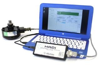
Excitation Voltage: Some users may need to change the excitation voltage or have a specific requirement for a 10V dc excitation to be applied to the sensor.
Choosing the right indicator is many times a matter of personal preferences. Choose the indicator that meets your needs with the best Non-Linearity and stability specifications.
Morehouse makes different indicators that meet various criteria mentioned above. If you need a rugged, battery-powered indicator with at least 50,000 counts of resolution, our G501F is an excellent choice. If you need a stable system and can carry a laptop with you, the Morehouse HADI may make the most sense. Finally, if you need a system where you must have a live display, use a computer, and need a 10V excitation source, the Morehouse 4215 would be a great option. We have a lot more information about these products and other topics as well on our website.
Glossary of Terms
This section contains a glossary of common terms in force measurement. It is important to have these for reference because most of these terms are used when speaking about characteristics of load cells, discussions on measurement uncertainty and calibration standards.
ASTM E74 – Standard Practices for Calibration and Verification for Force-Measuring Instruments: ASTM E74 is a practice that specifies procedures for the calibration of force-measuring instruments.5
Best existing force-measuring instrument (ILAC P14): “The term ‘best existing device’ is understood as a force-measuring instrument to be calibrated that is commercially or otherwise available for customers, even if it has a special performance (stability) or has a long history of calibration [1].” For force calibrations, this is often a very stable force transducer (load cell) and indicator with enough resolution to observe differences in repeatability conditions.
Calibration and Measurement Capability or CMC: “A CMC is a Calibration and Measurement Capability available to customers under normal conditions: a) as described in the laboratory’s scope of accreditation granted by a signatory to the ILAC Arrangement; or b) as published in the BIPM key comparison database (KCDB) of the CIPM MRA [1].”
Environmental Factors: Environmental conditions, such as temperature, influence the force transducer output. The most common specification is the temperature effect found on the force-measuring instrument’s specification sheet. It is important to note that any deviation in environmental conditions from the temperature that the force-measuring instrument was calibrated at must be accounted for in the measurement uncertainty, using the user’s force transducer measurements. For example, the laboratory calibrated a force-measuring instrument at 23 °C. The force-measuring instrument is then used from 13-33 °C or ±10 °C from the calibration. Based on the manufacturer’s specification, this temperature variation could cause an additional change on the force output by 0.015 % reading per °C, or 0.15 % reading for ±10°C. This number is typically found on the force transducer’s specification sheet as Temperature: Effect on Sensitivity, % Reading/100 °C or °F. The value will vary depending on the force transducer used. The example uses a common specification found for most shear-web type force transducers.
5 https://www.astm.org/e0074-18e01.html
Cal Lab: The International Journal of Metrology
29 Oct • Nov • Dec 2022
METROLOGY 101
Figure 12. High Accuracy Digital Indicator (HADI)
METROLOGY 101
Force Units: A force unit can be any unit representing a force. Common force units are N, kgf, lbf. The SI unit for force is N (Newton).
Hysteresis: The phenomenon in which the value of a physical property lags changes in the effect causing it, as for instance when magnetic induction lags the magnetizing force. For force measurements, hysteresis is often defined as the algebraic difference between output at a given load descending from the maximum load and output at the same load ascending from the minimum load. Normally, it is expressed in units of % full scale and calculated between 40 - 60 % of full scale.
ISO 376 - Calibration of force proving instruments used for the verification of uniaxial testing machines: ISO 376 is an International Standard that specifies a method for the calibration of force-proving instruments used for the static verification of uniaxial testing machines (e.g., tension/compression testing machines) and describes a procedure for the classification of these instruments.6
Lower limit factor (LLF): This is an ASTM specific term. The ASTM E74 standard uses a method of least squares to fit a polynomial function to the data points. The standard deviation of all the deviations from the predicted values by the fit function versus the observed values is found by taking the square root of the sum of all the squared deviations divided by the number of samples minus the degree of polynomial fit used minus one. This number is then multiplied by a coverage factor (k) of 2.4 and then multiplied by the average ratio of force to deflection from the calibration data. The LLF is a statistical estimate of the error in forces computed from the calibration equation of a force-measuring instrument when the instrument is calibrated in accordance with this practice.
Metrological traceability (JCGM 200:2012, 2.41): Property of a measurement result whereby the result can be related to a reference through a documented unbroken chain of calibrations, each contributing to the measurement uncertainty.
Non-Linearity: The quality of a function that expresses a relationship that is not one of direct proportion. For force measurements, Non-Linearity is defined as the algebraic difference between the output at a specific load and the corresponding point on the straight line drawn between the outputs at minimum load and maximum load. Normally, it is expressed in units of % of full scale and calculated between 40 - 60 % of full scale.
6 https://www.iso.org/obp/ui/#iso:std:iso:376:ed-4:v1:en
Non-Repeatability (per force transducer specification and not JCGM 200:2012): The maximum difference between output readings for repeated loadings under identical loading and environmental conditions. Normally expressed in units as a % of rated output (RO).
Other Force Measurement Errors: Most forcemeasuring instruments are susceptible to errors from misalignment, not exercising the force-measuring instrument to full capacity, and improper adapter use. There will be additional errors in almost all cases if the end user fails to have the force-measuring instrument calibrated with the same adapters being used in their application. Other errors may include temperature change under no-load conditions. Errors from loading equipment not being level, square and rigid can have significant contributions.
Primary Standard: Per ASTM E74, a deadweight force is applied directly without intervening mechanisms such as levers, hydraulic multipliers, or the like whose mass has been determined by comparison with reference standards traceable to the International System of Units (SI) of mass. Note: Weights used for force measurement require the correction for the effects of local gravity and air buoyancy and must be adjusted to within 0.005 % of nominal force value. The uncertainty budget for primary standards also needs to consider possible force-generating mechanisms other than gravity and air buoyancy, including magnetic, electrostatic, and aerodynamic effects.
Rated Output or RO: The output corresponding to capacity, equal to the algebraic difference between the signal at “(minimal load + capacity)” and the signal at minimum load.
Reference Standard(s) Calibration Uncertainty: This is usually the measurement uncertainty in the calibration of the reference standard(s) used to calibrate the force-measuring instrument.
Reference Standard(s) Stability: The change in the output of the reference standard(s) from one calibration to another. This number is found by comparing multiple calibrations against one another over time. If the instrument is new, the suggestion is to contact the manufacturer for stability estimation on similar instruments.
Repeatability condition of measurement, repeatability condition (JCGM 200:2012, 2.20): The “condition of measurement, out of a set of conditions that includes the same measurement procedure,
Lab: The International Journal of Metrology
30 Oct • Nov • Dec 2022
Cal
METROLOGY
same operators, same measuring system, same operating conditions, and same location, and replicate measurements on the same or similar objects over a short period of time [3].”
Measurement repeatability, Repeatability (JCGM 200:2012, VIM 2.21): “Measurement precision under a set of repeatability conditions of measurement.”
Repeatability can be calculated by taking the sample standard deviation of a series of at least two measurements at the same test point (three or more are recommended). The overall repeatability of more than one group of data is calculated by taking the square root of the average of variances, which is also known as pooled standard deviation. The purpose of this test is to determine the uncertainty of force generation in a force calibrating machine or test frame. For laboratories testing multiple ranges, it is recommended that the measurement sequence takes a point for every 10% of the ranges they calibrate.
Take for example, a laboratory performing calibrations from 10 N through 10,000 N, where the ranges calibrated may be 10 N - 100 N, 100 N - 1,000 N, and 1,000 N – 10,000 N. Recommended practice would be to take test points at 10, 20, 30, 40, 50, 60, 70, 80, 90, 100, 200, 300, 400, 500, 600, 700, 800, 900, 1,000, 2,000, 3,000, 4,000, 5,000, 6,000, 7,000, 8,000, 9,000, and 10,000 N.
For this application, zero should never be considered as a first test point. A force-measuring instrument should not be used to calibrate other force-measuring instruments outside the range it was calibrated over. A force-measuring instrument calibrated from 10 % through 100 % of its range may not be capable of calibrating force-measuring instruments outside of this range.
Resolution (JCGM 200:2012, VIM 4.14): The “smallest change in a quantity being measured that causes a perceptible change in the corresponding indication.”
Resolution of a Displaying Device (JCGM 200:2012, VIM 4.15): The “smallest difference between displayed indications that can be meaningfully distinguished.”
Reproducibility condition of measurement, reproducibility condition (JCGM 200:2012, VIM 2.24): The “condition of measurement, out of a set of conditions that includes different locations, operators, measuring systems, and replicate measurements on the same or similar objects.”
101
Measurement reproducibility, Reproducibility (JCGM 200:2012, VIM 2.25): “Measurement precision under reproducibility conditions of measurement.”
Reproducibility calculations between technicians can be found by taking the standard deviation of the averages of the same test point taken multiple times (multiple groups). There are other acceptable methods for determining reproducibility, and it is up to the end user to evaluate their process and determine if the method presented makes sense for them. For guidance on Repeatability and Reproducibility, the user should consult ISO 5725 Parts 1 - 6.
Secondary force standard (ASTM E74, Section 3.1.3): An instrument or mechanism, the calibration of which has been established by comparison with primary force standards.
Static Error Band: The band of maximum deviations of the ascending and descending calibration points from a best fit line through zero OUTPUT. It includes the effects of NON-LINEARITY, HYSTERESIS, and non-return to MINIMUM LOAD. Normally expressed in units of %FS.
Conclusion
We covered the basics about selecting the right equipment used in force calibration and knowing the proper terminology. Refer to our e-book, Force Calibration for Technicians & Quality Managers, that covers more advanced applications, as well as other guidance documents and tools that can add to your knowledge base at https://mhforce.com/ documentation-tools/. If you have any questions, don’t hesitate to reach out and contact us. Visit us at www.mhforce.com.
References
[1] ILAC-P14:09/2020, ILAC Policy for Measurement Uncertainty in Calibration. https://ilac. org/?ddownload=123348
[2] ISO 376:2011 Metallic materials – Calibration of force-proving instruments used for the verification of uniaxial testing machines. https://www.iso.org/obp/ ui/#iso:std:iso:376:ed-4:v1:en
[3] (VIM), 3rd Ed., JCGM 2012. International vocabulary of metrology – Basic and general concepts and associated terms. https://www.bipm.org/documents/20126/2071204/ JCGM_200_2012.pdf/
Cal Lab: The International Journal of Metrology
31 Oct • Nov • Dec 2022
Effects of Impurities on the Freezing Plateau of the Triple Point of Water
Xiaoke Yan, Jintao Zhang, Yuning Duan National Institute of Metrology (NIM)
Wei Wang Beijing University of Technology Xiaoming Hao University of Science and Technology Beijing
The influence of impurities on the shape of the freezing curves of the triple point of water (TPW) in three small TPW cells was investigated using the freezing curve analysis method. We describe the procedure for preparing outer ice mantles in small TPW cells, for obtaining freezing plateaus, and for comparing the results between the old cell (s/n: 021) and the new cells (s/n: 001 and s/n: 008). The experimental results show that the maximum influence of impurities on the observed phase-transition temperature of water in the cell (s/n: 021) is approximately 0.2 mK below the peak temperature of the freezing plateau during freezing. Also, jagged temperature fluctuations were observed near the end of the freezing plateau in the old cell. However, these phenomena did not appear in the freezing plateaus of the new small cells. The equilibrium temperature realized with the old cell is 2.3 mK lower than that of the new cells, possibly due to excessive residual air. Therefore, assessing the effects of impurities on the TPW using an outer sheath method similar to that used in obtaining the fixed points of other metals is useful. Additionally, an estimated total mole fraction impurity concentration can be determined using Raoult's Law and the first cryoscopic constant for water.
Introduction
The triple point of water (TPW) is the sole reference point for both the Thermodynamic Temperature Scale and the International Temperature Scale of 1990 (ITS90) [1]. The TPW is realized using TPW cells made of borosicilate or quartz glass. Research [2-7] shows that impurities from the glass containers can gradually dissolve into the water with time influencing its phase-transition temperature. Hence, impurity is a critical factor affecting the temperature realized by TPW cells. In order to reduce the uncertainty arising from impurities in the realization of the TPW at the highest level of accuracy, investigating the effects of impurities on the triple point temperature of water is critical.
Several national metrology institutes (NMIs), specially, the National Research Council of Canada (NRC) [3], the Nederlands Meetinstituut van Swinden Laboratorium (NMi-VSL) [8], the National Institute of Standards and Technology (NIST) [9], and
the National Metrology Institute of Japan (NMIJ) [10], have applied the Inductively Coupled Plasma Mass Spectrometry (ICPMS) to analyze impurities in water.
The freezing point temperature depresssion and the long-term drift of TPW cells are mainly ascribed to dissolution processes including leaching and etching [3-8]. The aging of borosilicate cells is initially very slow, and dominated by leaching, but as the cells age, etching becomes dominant, and the drift rate increases exponentially.
Since impurities are dependent on their concentrations and their properties in fixed point cells, they affect both the fixed-point temperature and the shape of the freezing and melting plateaus [11-13]. The effects of impurities on the metal fixed points of silver [14, 15], aluminum [16, 17], zinc [18], and tin [19] have been widely investigated. In this paper, we report an investigation into the effects of impurities on the freezing curves of small TPW cells conducted at the National Institute of Metrology (NIM), China.
32 Oct • Nov • Dec 2022 Cal Lab: The International
Journal of Metrology
Effects of Impurities on the Freezing Plateau of the Triple Point of Water Xiaoke Yan, Jintao Zhang, Yuning Duan, Wei Wang, Xiaoming Hao
Experiment
Small TPW Cells
Three small TPW cells (s/n: 001, s/n: 008, and s/n: 021), as shown in Figure 1, were used for this investigation. The cells were made of borosilicate glass. When the cells were shaken, a very sharp click was produced, indicating extremely low residual air in the cells. The old cell (s/n: 021) was sealed before 2000, and some floating impurities were visible in this cell. Additionally, water hammer test for the old cell indicated that it contained some residual air. However, the new cells (s/n: 008 and s/n: 001) were fabricated in 2008 in accordance with the NIM’s new production procedure [20]. The old cell (s/n: 021) had the same dimensions as the new cells (s/n: 001 and s/n: 008). However, no floating impurities were observable in the new cells.
Automated Maintenance Apparatus
Based on thermoelectric and heat pipe technologies, an automated maintenance apparatus for realizing the TPW was developed, as shown in Figure 2. The apparatus fulfills automatically freezing dendritic ice crystals and maintains them in a mushy state. Detailed information on the apparatus was described previously [21].
Small TPW cell
Plastic cover
Small holes
Thermoelectric cooling module
Heat pipe radiator
Cooling fan
Aluminum container
Plastic holder
Stainless-steel sleeve Heater
Thermal insulation
Figure 1. Cross-sectional drawing of a small TPW cell.
Temperature Measurement System
The temperature measurement system contained a Guildline 6622A-XPS Automatic DCC Resistance Bridge (s/n 69547), one nominal 10 Ω standard resistor, a temperature controlled oil bath to keep the standard resistor at constant temperature, a Standard Platinum Resistance Thermometer (SPRT) (s/n: 95025), and a computer for data acquisition. In order to improve the temperature stability of the standard resistor, an annular water heat pipe thermostat was used to accommodate the standard resistor [22]. Using this heat pipe thermostat, the temperature stability over 24 hours was maintained to within 1 mK during measurement. The acquisition of bridge readings was carried out automatically by a programmed computer.
Outer Sheath Method
Supercooled high purity water can spontaneously transform into metastable mushy needle-like crystallites [23]. Also, the temperatures at which the phase changes occur depend on the cooling rate
Cal Lab: The International Journal of Metrology
33 Oct • Nov • Dec 2022
8 mm
45 mm O. D. 4 0
1 6 0 m
4
Figure 2. Schematic diagram of the automated maintenance apparatus.
I. D. Rubber foot
m m
m
0 m m Air-free water
Effects of Impurities on the Freezing Plateau of the Triple Point of Water
and on the impurities in the water: the more rapid the cooling rate and the greater the concentration of impurities in the water, the less the supercooling that causes the spontaneous phase transitions. Therefore, the supercooling in the old cell would be expected to be less than that in the new cells, because impurities in water would favor the creation of crystal nucleating sites.
Based on this principle, a mushy mixture of solid-liquid throughout the cell was obtained when recalescence occurred. Once obtained, the small TPW cells were maintained at 0 °C to stabilize the mush, and the mushy fine needle crystals adjacent to the wall of the cells thickened and transformed into an outer ice mantle with no visible cracks. A standard platinum resistance thermometer (s/n: 95025) at room temperature was inserted into the thermometer well to form an inner melt from the mushy crystals as soon as the spontaneous phase transitions happened. When the SPRT was in thermal equilibrium, measurements were started. The outer ice mantle advanced and thickened from the outside inward. The remaining metastable ice crystals were between the inner melt and the outer ice mantle [21, 23]. A schematic diagram of the ice mantle in the small TPW cell is illustrated in Figure 3.
Comparison of TPW between the Old Cell and the New Cells
The old cell (s/n: 021) was compared with the new cells (s/n: 001 and s/n: 008) using the same maintenance apparatus, temperature measuring system, and freezing procedure. While keeping them under the same freezing conditions in the automated maintenance apparatus, the shapes of the freezing curves were obtained, and the cells showed differences that appeared to be due to impurities. In this way, impurity effects on the freezing plateaus were able to be determined and evaluated applying Raoult’s Law and the first cryoscopic constant for water [11-13].
Results and Discussion
Freezing Experiments
The outer ice mantles in the small TPW cells were prepared using the outer sheath method. In this investigation, we conducted freezing experiments on three cells maintained at a temperature in the range from approximately 0 °C to -0.2 °C. Typical freezing curves for the cells are shown in Figures 4, 5, and 6. The freezing curves were obtained using the same apparatus. For the old cell (s/n: 021), a gradual temperature decrease was observed. This decrease may be attributable to an increase in the concentration of impurities in the water, due to the advancing frozen water front excluding the impurities as the outer ice mantle advanced inward. However, this phenomenon was not observed for the new cells (s/n: 008 and s/n: 001) with their lower impurity contents (Figures 5 and 6). These observations provide a visual view of the effects of impurities on the shape of the freezing plateaus.
The duration of freezing plateaus depends on the temperature difference between the set temperature and the triple point temperature of water; the smaller the temperature difference, the longer the duration of the freezing plateaus. In Figure 4, the set temperatures in 2008 and 2011 were 0 °C and -0.1 °C, respectively. Therefore, the duration of the freezing curve obtained in 2008 was longer than that obtained in 2011.
Additionally, the spontaneous crystallization temperatures for the cells were different, as listed in Table 1. This may be the result of differences in the performance of the thermo-electric cooling modules and cooling rates.
34 Oct • Nov • Dec 2022 Cal Lab: The
International Journal of Metrology
Figure 3. Schematic diagram of the TPW cell with an outer ice mantle.
Ice mantle
Inner melt
Metastable ice crystals
Xiaoke Yan, Jintao Zhang, Yuning Duan, Wei Wang, Xiaoming Hao
Effects of Impurities on the Freezing Plateau of the Triple Point of Water Xiaoke Yan, Jintao Zhang, Yuning Duan, Wei Wang, Xiaoming Hao
Resistance of SPRT (s/n: 95025), Ω Resistance of SPRT (s/n: 95025), Ω
August 26-27, 2008 0.1 mK
2 4 6 8 10 12 14 16 18 20 25 25886 25 25887 25 25888 25 25889 25 25890 25 25891 25 25892 25 25893 25 25894
Time, hours
Small TPW Cell (s/n: 021) 2 3 4 5 6 7 8 9 10 11 12 25 25938 25 25939 25 25940 25 25941 25 25942 25 25943 25 25944 25 25945 25 25946 Time, hours
June 4-5, 2011 Small TPW Cell (s/n: 021) 0 1 mK
Figure 4. Freezing curves of the small TPW cell (s/n: 021) obtained in 2008 and 2011.
Time Serial Number Resistance of SPRT at TPW, Ω
Temperature difference, mK
Maximum Temperature Depression, mK
Spontaneous Phase Transition Temperature, °C
Aug. 26-27, 2008 021 25.25891 -2.3 -0.2 -5.80 Sept. 16-17, 2008 008 25.25914 0.0 0.0 -6.41
Jun. 4-5, 2011 021 25.25943 -2.2 -0.2 -4.78 Jun. 3-4, 2011 001 25.25965 0.0 0.0 -8.60
Feb.1-2, 2012 021 25.25965 -0.3 -4.69
Evaluation of Impurity Effects
Assuming that the impurities are only soluble in liquid water, the effects of impurities can be assessed using Raoult’s Law. That is, the freezing point temperature depression (Δ T ) attributable to impurities can be expressed by the following equation:
ΔT = Tpure − Tobs = c1 / A
in which T pure and T obs are the freezing-point temperature of pure water and the observed equilibrium temperature of water, respectively; c1 is the mole fraction impurity concentration; and A is the first cryoscopic constant. A is given by the relationship:
Table 1. Experimental results. (1) (2)
A = L / R
in which L is the molar heat of fusion and R is the molar gas constant. Here, for water, L=6.008 kJ/mol; A=0.00968 K-1 [11].
For the old cell, the maximum temperature depression of the freezing plateau of water was
approximately 0.2 mK. Based on equation (1) and the first cryoscopic constant for water, the total mole fraction impurity concentration can be calculated as 1.936×10⁻⁶. Using this method, the estimated impurity concentrations can be compared between the TPW cells.
Temperature Fluctuations Near the End of the Freezing Plateaus
Jagged temperature fluctuations appeared in the old cell (s/n: 021) near the end of each freezing plateau, as shown in Figure 7. The concentration of the impurities in the water around the thermometer well gradually increased as the outer ice mantle advanced inward. The diffusion of the impurities caused temperature oscillations in the old cell. However, this phenomenon was not observed in the new cells apparently due to lower concentrations of impurities. Therefore, such fluctuations can be used to assess impurity in the water in sealed cells. In addition, these fluctuations may feasibly be used as indicators that the freezing plateau is nearing the
Cal Lab: The International Journal of Metrology
35 Oct • Nov • Dec 2022
Effects of Impurities on the Freezing Plateau of the Triple Point of Water Xiaoke Yan, Jintao Zhang, Yuning Duan, Wei Wang, Xiaoming Hao
Resistance of SPRT (s/n: 95025), Ω Resistance of SPRT (s/n: 95025), Ω
September 16-17, 2008 0 1 mK
Small TPW Cell (s/n: 008)
0 2 4 6 8 10 12 14 16 18 20 22 25 25907 25 25908 25 25909 25 25910 25 25911 25 25912 25 25913 25 25914 25 25915 25 25916 25 25917 Time, hours
Figure 5. Freezing curve of the small TPW cell (s/n: 008) obtained in 2008.
s/n: 008). Impurities in water lowered the phasetransition temperature of the water by at most 0.3 mK. Therefore, the remaining temperature difference may be explained by a poor hammer effect (excessive air).
Conclusions
June 3-4, 2011 Small TPW Cell (s/n: 001)
0 1 mK
0 2 4 6 8 10 12 14 16 18 20 25 25959 25 25960 25 25961 25 25962 25 25963 25 25964 25 25965 25 25966 25 25967 25 25968 25 25969 Time, hours
Figure 6. Freezing curve of the small TPW cell (s/n: 001) obtained in 2011.
end. In other words, the freezing experiments should stop as soon as temperature oscillations appear during freezing.
Comparison Results
The comparison results between the old cell and the new cells are shown in the Table 1. It can be seen that the peak freezing temperature realized in the old cell (s/n: 021) is approximately 2.3 mK lower than the peaks in the new cells (s/n: 001 and
The effects of impurities on the triple point temperature of water and on the shape of the freezing plateau were investigated using a freezing curve analysis method. A conclusion can be drawn that the impurities changed the shape of the freezing plateau of the water in the old cell and lowered the phase-transition temperature. The maximum freezing point depression of the plateau obtained in the old cell (s/n: 021) was approximately 0.2 mK below the peak temperature of the freezing curve. Assuming that Raoult’s law holds and using the first cryoscopic constant for water, the maximum freezing range observed in the old cell (s/n: 021) suggests an impurity content of 1.936×10⁻⁶.
Jagged temperature fluctuations near the end of the freezing plateau in the old cell were observed. This phenomenon appears to be related to the diffusion of impurities.
Acknowledgments
We are indebted to Researchers Peter Steur of INRiM and Qi Zhao of NIM for their valuable discussions and suggestions. Also, we thank Researchers Chi Wang and Tiejun Wang of NIM for their support of this research. Additionally, we are indebted to Profs. Edmund F. and Rhoda E. Perozzi for modifications and discussions of the English and the content of this paper.
February 1-2, 2012 25 25963 Resistance of SPRT (s/n: 95025), Ω Resistance of SPRT (s/n: 95025), Ω
20 5 21 0 21 5 22 0 22 5 23 0 25 25883 25 25884 25 25885 25 25886 25 25887 25 25888 25 25889 25 25890 25 25891 25.25892 25 25893 Time, hours
August 26-27, 2008 0.1 mK
25 25964 25 25965 25 25966 25 25967 Time, hours
Small TPW Cell (s/n: 021) 0.1 mK
Small TPW Cell (s/n: 021) 8.0 8.5 9.0 9.5 10.0 25 25957 25 25958 25 25959 25 25960 25 25961 25.25962
Figure 7. Temperature fluctuations observed near the end of the freezing plateau of the cell (s/n: 021) in 2008 and 2012.
36 Oct • Nov • Dec 2022 Cal Lab: The International Journal of Metrology
Effects of Impurities on the Freezing Plateau of the Triple Point of Water Xiaoke Yan, Jintao Zhang, Yuning Duan, Wei Wang, Xiaoming Hao
References
[1] Preston-Thomas H., Metrologia, 27, 3-10 (1990).
[2] Hill, K. D., “ A Comparison of Triple Point of Water Cells” in Proceedings of the International Conference of the Temperature and Thermal Measurements (TEMPBEIJING’97), edited by B. Y. Zhang, Standards Press of China, Beijing, 1997, pp.10-15.
[3] Hill, K. D., “ Triple Point of Water Cells and the Solubility of Borosilicate Glass” in Proceedings of 7th International Symposium on Temperature and Thermal Measurements in Industry and Science ( TEMPMEKO’99), edited by J. F. Dubbeldam, M. J. de Groot, NMi Van Swinden Lab., Delft, 1999, pp. 68-73.
[4] Hill, K. D., “Long-term Drift in Triple Point of Water Cells,” Document CCT/2000-5, 2000.
[5] Hill, K. D., Metrologia, 38, 79 -82 (2001).
[6] Mendez-Lango, E., “A non-destructive Method to Evaluate the Impurity Content in Triple Point of Water Cells” in Proceedings of 8th International Symposium on Temperature and Thermal Measurements in Industry and Science ( TEMPMEKO2001), edited by B. Fellmuth, et. al., VDE Verlag, Berlin, 2002, pp. 465470.
[7] Yan, X. K., Ma C. F., Zhang, Z., Wu, H. L., Qiu, P., Feng, Y. L., Zhang, J. T., Duan, Y. N., International Journal of Thermophysics, 29, 815-824 (2008).
[8] Peruzzi, A., Kerkhof, O., De Groot, M. J., International Journal of Thermophysics, 28, 1931-1940 (2007).
[9] Strouse, G. F., Zhao, M., International Journal of Thermophysics, 28, 1913-1922 (2007).
[10] Tamba, J., Sakai, M., Kishimoto, I, Arai, M., International Journal of Thermophysics, 29, 1749-1760 (2008).
[11] Mangum, B. W., Bloembergen, P., Fellmuth, B., Marcarino, P., Pokhodun, A. I., “On the Influence of Impurities on the Fixed-Point Temperatures,” CCT document CCT99-11, 1999.
[12] Fellmuth, B., Hill, K. D., Bloembergen, P., De Groot, M., Hermier, Y., Matveyev, M., Pokhodun A., Ripple, D., Steur, P. P. M., “Methologies for the Estimation of Uncertainties and Correction of Fixed-Point Temperatures Attributable to the Influence of Chemical Impurities,” CCT document CCT/05-08, 2005.
[13] Strouse, G. F., “ Methods of Estimating the Impurity Uncertainty Comment for ITS-90 Fixed-Point Cells from the Ar TP to the Ag FP,” CCT document CCT/03-19, 2003.
[14] Ancsin, J., Metrologia, 38, 229-235, 2001.
[15] Widiatmo, J. V., Harada, K., Yamazawa, K., Arai, M., International Journal of Thermophysics, 29, 158-170 (2008).
[16] Ancsin, J., Metrologia, 40, 36-41, 2003.
[17] Widiatmo, J. V., Harada, K., Yamazawa, K., Arai, M., Metrologia, 43, 561-572, 2006.
[18] Ancsin, J., Metrologia, 44, 303-307, 2007.
[19] Fellmuth, B., Hill, K. D., Metrologia, 43, 71-83, 2006.
[20] Yan, X., Qiu, P., Wang, Y., Wu, H., Feng, Y., and Zhang, “NIM Development of the Triple Point of Water Cells of High Quality,” in Proceedings of 9th International Symposium on Temperature and Thermal Measurements in Industry and Science (TEMPMEKO2004), Part 1, D. Zvizdic, ed. Laboratory for Process Measurement, Cavtat-Dubrovnik, 2005, pp. 283-288.
[21] Yan, X. K., Duan, Y. N., Yang, J. H., Li, J., International Journal of Thermophysics, 32, 481-493 (2011).
[22] Yan, X. K., Duan, Y. N., Zhang, J. T., Wang, W., Wang, L., Li, J., “Improvement in Temperature Stability of Standard Resistors Using Heat Pipe Technology,” In Temperature: Its Measurement and Control in Science and Industry, edited by J. F. Strouse et al., AIP, Los Angeles, 2012, 8.
[23] Cox, J. D., Vaughan, M. F., “ Temperature Fixed Points: Evaluation of Four Types of Triple Point Cell,” In Temperature: Its Measurement and Control in Science and Industry, edited by J. F. Schooley, AIP, New York, 1982, 5, pp. 267-280.
Xiaoke Yan (corresponding author: yanxk@nim. ac.cn), Jintao Zhang, and Yuning Duan of National Institute of Metrology (NIM), Beijing, China; Wei Wang of Beijing University of Technology, Beijing, China; and Xiaoming Hao of University of Science and Technology Beijing, China.
The preceeding was reproduced from “Effects of impurities on the freezing plateau of the triple point of water,” AIP Conference Proceedings 1552, 209 (2013); https://doi. org/10.1063/1.4821379, with the permission of AIP Publishing. It was included as part of the proceedings of the Ninth International Symposium (ITS9), 19-23 March 2012, Los Angeles, California, USA, and is republished here in anticipation of the upcoming ITS10, 3-7 April 2023 in Anaheim, California. For more information, visit https://its10.msc-conf.com.
Cal Lab: The International Journal of Metrology
37 Oct • Nov • Dec 2022
Practitioner’s Perspective on the GUM Revision, Part II: Examples and Resolutions to the Ballico Paradox
Hening Huang Teledyne RD Instruments (retired)
This paper is the second one (Part II) in a series of two papers (Part I and Part II) designated to provide practitioner’s perspective on the GUM revision. Part I has discussed two key problems and their solutions. This paper (Part II) examines four examples of the GUM in detail, using the two alternative approaches described in Part I to calculate the expanded uncertainty, and compares to GUM’s WS-t approach. It also describes the resolutions to the Ballico paradox due to GUM’s WS-t approach.
1. Introduction
This paper (Part II of a series of two papers) continues our discussion in Part I (Huang 2022) on practitioner’s perspective on the GUM revision. In Part I, we pointed out that the (current) GUM has two key problems: (1) inconsistency in GUM’s two definitions of measurement uncertainty, and (2) limitations of GUM’s WS-t approach for calculating the expanded uncertainty. Especially, GUM’s WS-t approach leads to the Ballico paradox, which is unacceptable in practice. As discussed in Part I, the first problem can be solved by defining ‘uncertainty of measurement’ as the ‘probabilistic error bound’ based on the law of error. The second problem can be solved by either of the two alternative approaches described in Part I.
In this paper (Part II), we will focus on applying the two alternative approaches to four real-world examples given in the GUM. Annex H of the GUM (JCGM 2008) provides six examples, numbered H.1, H.2,…, H.6, to illustrate the basic principles for evaluating measurement uncertainty. We only consider GUM’s examples H.2, H.3, H.4, and H.6 here. Example H.5 is an analysis of variance (ANOVA), which has nothing to do with the expanded uncertainty. Example H.1 was examined in detail by Huang (2018), so it is not considered here. Notice that the GUM only computes the combined standard uncertainty (CSU) u c(y)for these four examples. In this study, we compute the CSU u c ( y ) , modified
CSU u c ′(y), and expanded uncertainty at the nominal coverage probability p=95% using the two alternative approaches. For comparison, we also compute the expanded uncertainty using GUM’s WS-t approach. The resolutions to the Ballico paradox using the two alternative approaches are also described.
In the following, section 2 briefly recaps GUM’s WS- t approach and two alternative approaches. Sections 3 to 6 discuss four GUM examples H.2, H.3, H.4, and H.6. Section 7 summarizes six examples of the GUM. Section 8 shows the resolutions to the Ballico paradox. Section 9 presents conclusion and recommendation.
2. Brief Recap of GUM’s WS-t Approach and Two Alternative Approaches
The combined standard uncertainty (CSU) u c(y) of the estimate y of the measurand Y is written as
where c i is the sensitivity coefficient, s i is the sample standard deviation and n i is the number of observations of the ith Type A quantity, NA is the number of the Type A quantities, N is the total number of influence quantities (Type A and Type B), and r i,j is the estimated correlation coefficient.
38 Oct • Nov • Dec 2022 Cal Lab: The International Journal of Metrology
u c (y) = √ ∑ i 1 NA ci2 si2 ni + ∑ k=NA+1 N ck2 uB,k 2 + 2∑ i 1 NA 1 ∑ j+1 NA ci cj si √ ni sj √ nj ri,j (1)
Hening Huang
We assume that only Type A quantities may be correlated, and there is no correlation between a Type A quantity and a Type B quantity, or between two Type B quantities.
GUM’s WS-t approach for calculating the expanded uncertainty is written as where t p,ν eff is the t-value at the nominal coverage probability p, νeff is the effective DOF for the CSU u c (y), which can be calculated according to the WelchSatterthwaite formula
Then, the second alternative approach is written as
For the special case where only one Type A influence quantity is involved in the measurement model, i.e. Y = X , the effective DOF ν e f f reduces to n-1 and the CSU reduces to the Type A SU s √ n Accordingly, GUM’s WS-t approach reduces to
And the two alternative approaches give the same estimate of the Type A expanded uncertainty. That is
where νi is the DOF associated with the ith uncertainty component ui
The first alternative approach is written as where c4,eff is the bias correction factor for the CSU u c (y), which is written as where Г(.) stands for Gamma function. The bias correction factor can be calculated using an Excel spreadsheet. However, it should be noted that Excel’s built-in Gamma function is valid for νeff≤342; it fails for νeff>343. For νeff>343, it is reasonable to use c4,νeff
3. Example H.2: Simultaneous Resistance and Reactance Measurement
= 1
The second alternative approach requires the modified CSU u c ′ (y), which is written as
The GUM describes the following problem. “The resistance R and the reactance X of a circuit element are determined by measuring the amplitude V of a sinusoidally-alternating potential difference across its terminals, the amplitude I of the alternating current passing through it, and the phase-shift angle ϕ of the alternating potential difference relative to the alternating current. Thus the three input quantities are V, I, and ϕ and the three output quantities — the measurands — are the three impedance components R, X, and Z. Since Z2 = R2 + X2, there are only two independent output quantities (JCGM 2008, p85).” Five independent sets of simultaneous observations of the three quantities V, I, and ϕ are obtained under similar conditions. This example only considers the random variations of the observations. Therefore, it is a pure Type A evaluation of uncertainty.
where c4,ni 1 is the bias correction factor for the Type A SU s √ ni , which is written as
The GUM uses two different approaches to calculate the CSU for all three measurands, R, X, and Z. Approach 1 is based on the law of propagation of uncertainty. Approach 2 is a direct Type A analysis of the measurement data. Approach 2 is much simpler than approach 1. The GUM shows that the two approaches yield essentially the same numerical results. We follow GUM’s approach 2 and consider the measurand Z only. In approach 2, a value for Z is
Cal Lab: The International Journal of Metrology
39 Oct • Nov • Dec 2022
U p,GUM = t p,ν eff u c
ν eff = u c 4(y) ∑ i=1 N c 4 ui4 νi = [∑ i 1 N ci2 ui2] 2 ∑ i 1 N c 4 u 4 νi
U p,1 = z p u c(y) c4,ν eff
c4,ν eff = √ 2 ν eff Γ(ν eff + 1 2 ) Γ(ν eff 2 )
= √ ∑ i=1 NA ci2 si2 c4,ni 1 2 ni + ∑ k=NA+1 N ck2 uB,k 2 + 2∑ i=1 NA 1 ∑ j+1 NA ci cj si c4 ni 1 √ ni sj c4 nj 1 √ nj ri,j uc ′ (y)
c4,ni 1 = √ 2 ni 1 Γ(n 2 ) Γ(n 1 2 ) (7) U p,2 = z p u c ′
U p,GUM = t p,n 1 s √ n
U p,1 = U p,2 = z p s c4,n 1 √ n
(y) (2)
(3)
(4)
(5)
(6)
(y) (8)
(9)
(10) Practitioner’s Perspective on the GUM Revision, Part II: Examples and Resolutions to the Ballico Paradox
Practitioner’s Perspective on the GUM Revision, Part II: Examples and Resolutions to the Ballico Paradox Hening Huang
V (V) I (mA) Z (Ω)
1 5.007 19.663 254.64
2 4.994 19.639 254.29
3 5.005 19.640 254.84
4 4.990 19.685 253.49
5 4.999 19.678 254.04
Table 1. Five observations of the quantities V and I, and the calculated values for the measurand Z in example H.2.
computed according to Z = V / I from each set of the data for V and I, yielding a set of five values of Z (Table 1).
The data for Z gives the arithmetic mean 254.260 Ω and the sample standard deviation s=0.528 Ω. The arithmetic mean is taken as the best estimate of Z. That is, z=254.260 Ω. In the GUM, the experimental standard deviation of the mean is taken as the CSU of z. That is, u c(z) = s √ n = 0.528 / √ 5 =0.236 Ω, which is the Type A SU. The effective DOF νeff = 4 and the corresponding t-value at p=95% t95,4 = 2.776. Then, for this particular case that there is only one influence quantity involved in the measurement model Y = Z , GUM’s WS- t approach gives the expanded uncertainty
U95,GUM = t95,4 u c(z) = 2.776 × 0.236 = 0.656 Ω.
The bias correction factor for the CSU is c4,νeff
= 0.940 at νeff = 4. Then, the first alternative approach gives
U95,1 = z95 c4,4 u c(z) = 1.96 0.940 × 0.236 = 0.493 Ω.
The bias correction factor for the Type A SU is c 4 , n 1 = 0.940 at n = 5 . The modified CSU u c ′ ( y ) = s c 4,4 √ n = 0.528 0.940 × √ 5 = 0.251 Ω. Then, the second alternative approach gives
U95,2 = z95 u c ′ (y) = 1.96 × 0.251 = 0.493 Ω.
The result is the same as the first alternative approach. This is expected as Eq. (10) suggests.
4. Example H.3: Calibration of a Thermometer
This example considers the following linear calibration curve for a thermometer (GUM’s formula (H.12)) (i.e. measurement model)
where b ( t ) is the correction to be applied to the thermometer for any value t of the temperature, t0 is the reference temperature, y1 and y2 are respectively the intercept and slope of the calibration curve. The expression for the CSU of b(t) is written as (refer to GUM’s formula (H.15))
where u(y1) is the SU of y1, u(y2) is the SU of y2, and r ( y1, y2) is the estimated correlation coefficient. Note that in this example, the two influence quantities y1 and y2 are correlated.
A total of 11 datasets for temperature measurement are used to obtain a linear calibration curve for the thermometer (data are shown in Table H.6 of the GUM (JCGM 2008, p91)). Taking t0 = 20 °C as the reference temperature, the GUM gives the following statistics from the data (JCGM 2008, p.90): y1=−0.1712 °C, y2=0.00218, r(y1, y2 )=−0.930, u(y1)=0.0029 °C, and u(y2)=0.00067.
In this example, the GUM considers the case that one requires the thermometer correction and its uncertainty at t = 30 °C. Substituting y1=−0.1712 °C, y2=0.00218, t0 = 20 °C and t = 30 C in Eq. (11) yields b (30 °C) = 0.1494 °C.
Substituting u(y1)=0.0029 °C, u(y2)=0.00067 °C, r(y1, y2 )=−0.930, t = 30 °C and t0 = 20 °C in Eq. (12) yields u c[b (30 °C)] = 0.0041 °C.
The effective DOF for the CSU u c[b (30 °C)] can be calculated using the Welch-Satterthwaite formula, Eq. (3), and assuming that y1 and y2 have a DOF of 11-2=9. This gives
b(t) = y1 + y2(t t0) (11) u c[b(t)] (12) = √ u 2(y1) + (t t0) 2 u 2(y2) + 2(t t0)u( y1)u( y2)r( y1, y2) νeff = ( 0.0029 2 + (30 20) 2 0.00067 2) 2 0.0029 4 9 + (30 20) 4 0.00067 4 9 = 12.
The t-value for νeff = 12 at p=95% is t95,12 = 2.179 Then, GUM’s WS-t approach gives the expanded uncertainty
40 Oct • Nov • Dec 2022 Cal Lab: The
International Journal of Metrology
U95,GUM = t95,4 u c[b(30° C)]= 2.179 × 0.0041 = 0.0090 °C.
ratio of the background-corrected counting rate R x and decay-corrected counting rate R s .
The bias correction factor for the CSU is c4,νeff
= 0.9794 at νeff = 12. Then, the first alternative approach gives
U95,1 = z95 c4 ν ff u c[b(30° C)] = 1.96 0.9794 × 0.0041 = 0.0083 °C.
The bias correction factor for the Type A SU is c4,9 = 0.9727. The modified CSU of b(t) is calculated as
Then, the second alternative approach gives
U95,2 = z95 u c ′ [b(t)] = 1.96 × 0.0042 = 0.0083 °C.
5. Example H.4: Measurement of Activity
This example considers the unknown radon (222Rn) activity concentration in a water sample. Again, the GUM uses two approaches in the analysis and shows that the two approaches yield essentially the same numerical results. We follow GUM’s approach 2. The measurement model corresponding to approach 2 is written as where A x is the measurand and is defined as the unknown activity concentration of the sample at the reference time t = 0, A s is activity concentration of the standard at the reference time t = 0, m s is mass of the standard solution, m x is the mass of the sample aliquot, and R is the sample mean of R that is the
The estimates for A s, m s, and m x and associated SUs are given in the GUM; they are the Type B quantities. The datasets for R x and R s are obtained from six cycles of measurement of the three counting sources and shown in Table H.8 of the GUM (JCGM 2008, p96). A value for R is computed according to R =R x/ R s from each set of the data for R x and R s, yielding a set of six values of R, from which the sample mean R and associated SU can be calculated. Therefore, R is a Type A quantity. Table 2 summaries the estimate, associated SU and DOF, and bias correction factor for each of these four influence quantities. Note that the DOF for A s, m s, or m x is infinity because they are Type B quantities. Accordingly, no bias correction is required for these Type B quantities, i.e. c4,∞ = 1. Readers are referred to the GUM (JCGM 2008) for details on these quantities and the measurement.
Substituting the estimates of the influence quantities shown in Table 4 into Eq. (13) yields A x = 0.4304 Bq/g.
All the influence quantities are uncorrelated. The expression for the CSU (relative) of A x is written as (refer to GUM’s formula (H.23b)
Substitute the estimates and SUs shown in Table 2 into Eq. (14). Then, the CSU of A x is calculated as u c(A x) = 0.0084 Bq/g.
The effective DOF for the CSU of A x can be calculated using the Welch-Satterthwaite formula, Eq. (3). This gives νeff = 17.
Quantity Estimate SU Type DOF c 4,DOF As 0.1368 Bq/g 0.0018 Bq/g B ∞ 1 ms 5.0192 g 0.0050 g B ∞ 1 mx 5.0571 g 0.0010 g B ∞ 1 R 3.17 0.046 A 5 0.9515
Table 2. Estimate, associated SU and DOF, and bias correction factor for each of the four influence quantities in example H.4.
Cal Lab: The International Journal of Metrology
41 Oct •
•
Nov
Dec 2022
= √
u c ′ [b(t)]
u 2(y1) c4.9 2 + (t t0) 2 u 2(y2) c4.9 2 + 2(t t0) u(y1)u(y2) c4,9 c4,9 r(y1, y2) = √ 0.0029 2 0.9727 2 + (30 20) 2 0.00067 2 0.9727 2 + 2(30 20) 0.0029 × 0.00067 0.9727 × 0.9727 ( 0.93) = 0.0042 ° C. A x = A s m s m x R (13) u c( A x) A x = √ u 2( A s) A s 2 + u 2( m s) m s 2 + u 2( m x) m x 2 + u 2(R ) R 2 (14)
Practitioner’s Perspective on the GUM Revision, Part II: Examples and Resolutions to the Ballico Paradox Hening Huang
Practitioner’s Perspective on the GUM Revision, Part II: Examples and Resolutions to the Ballico Paradox Hening Huang
The t-value for νeff = 17 at p=95% is t95,17 = 2.11. Then, GUM’s WS-t approach gives the expanded uncertainty
U95,GUM = t95,17 u c(A x) = 2.110 × 0.0084 = 0.0178 Bq/g.
(refer to GUM’s formula (H.38))
The bias correction factor for the CSU is c4,νeff
= 0.9854 at νeff = 17. Then, the first alternative approach gives
U95,1 = z95 c4,ν ff u c(A x) = 1.96 0.9854 × 0.0084 = 0.0168 Bq/g.
The expression for the modified CSU (relative) of A x is written as
u c ′ ( A x) A x
= √ u 2( A s) c4,∞ 2 A s 2 + u 2( m s) c4,∞ 2 m s 2 + u 2( m x) c4,∞ 2 m x 2 + u 2(R ) c4,5 2 R 2 (15)
Substitute the estimates and SUs shown in Table 2, and c4,∞ = 1, c4,5 = 0.9515, into Eq. (15). Then, the modified CSU of A x is calculated as u c ′ (A x) = 0.0087 Bq/g.
Then, the second alternative approach gives U95,2 = z95 u c ′ ( A x) = 1.96 × 0.0087 = 0.0170 Bq/g.
6. Example H.6:
Measurements
on a Reference Scale: Hardness
In this example, the hardness of a sample block of material is determined on the scale “Rockwell C,” using a machine that has been calibrated against the national standard machine. The calibration is quite complex and involves seven influence quantities. Here, we use the same notations for these seven quantities as the GUM, but do not explain their meanings. Interested readers are referred to the GUM (JUGM 2008, p104-108) for details of the measurements and analysis.
The CSU u c (h) of the hardness of the sample block as measured by the calibration machine is written as
s 2( d k) δ 2 s av
Table 3 shows the values for the uncertainty components used in the GUM calculations. The DOFs associated with these quantities are derived from the information given in the GUM. The bias correction factors are calculated based on the DOFs. These data are also shown in Table 3.
Substituting the values in Table 3 into Eq. (16) yields u c (h) = 0.55 Rockwell scale unit.
The effective DOF of u c (h) is calculated using the Welch-Satterthwaite formula, Eq. (3). This gives νeff = 229.
The t-value for νeff = 229 at p=95% is t95,17 = 1.970. Then, GUM’s WS-t approach gives the expanded uncertainty
U95,GUM = t95,229 u c (h) = 1.970 × 0.55 = 1.092 Rockwell scale unit.
The bias correction factor for the CSU is c4,νeff
= 0.9989 at νeff = 229. Then, the first alternative approach gives U95,1 = z95 c4 ν ff u c (h) = 1.96 0.9989 × 0.55 = 1.087 Rockwell scale unit.
The expression for the modified CSU of h is written as
(17)
u c (h) = √ s 2( dk) 5 + δ 2 12 + s av 2 ( z s) m + s av 2 (z ) n + (xz′) 2 24 + u 2( Δ s) (16) u c ′ (h) = √ s 2( dk) c4,4 2 5 + δ 2 c4,∞ 2 12 + s av 2 ( z s) c4,m 1 2 m + s av 2 (z ) c4,n 1 2 n + (xz′) 2 c4,∞ 2 24 + u 2( Δ s) c4,∞ 2
2 ( z s) s av
2 ( z ) (xz′) 2 u 2( Δ s)
Value 0.452 0.12 0.102 0.112 (0.015×36.0)2 0.52 DOF 5-1 ∞ m 1 (m=6) n 1 (n=6) ∞ ∞ c 4 DOF c 4 4 = 0.94 c 4 ∞ = 1 c 4 5 = 0.9515 c 4 5 = 0.9515 c 4 ∞ = 1 c 4 ∞ = 1
Table 3. Values in (Rockwell scale unit)2 for the uncertainty components used in the GUM calculations, associated DOFs, and corresponding bias correction factors in example H.6.
Cal Lab: The International Journal of Metrology
•
•
42 Oct
Nov
Dec 2022
Practitioner’s Perspective on the GUM Revision, Part II: Examples and Resolutions to the Ballico Paradox
Hening Huang
Example ν eff t 95,ν eff
c 4,ν eff u c(y) u c ′ (y)
H.1 End-gauge calibration 16 2.120 0.9845 32 nm 33 nm
H.2 Simultaneous resistance and reactance measurement: Z=V/I (a) 4 2.776 0.940 0.236 Ω 0.251Ω
H.3 Calibration of a thermometer 12 2.179 0.9794 0.0041 oC 0.0042 oC
H.4 Measurement of activity (b) 17 2.110 0.9854 0.0084 Bq/g 0.0087 Bq/g
H.6 Measurement on a reference scale: hardness (c) 229 1.970 0.9989 0.55 RSU 0.56 RSU
G.4.1 Y=f(X1, X2, X3)=bX1X2X3 19 2.093 0.9869 1.03% 1.06%
Table 4. Effective DOF, t-value, bias correction factor for the CSU, CSU, and modified CSU for the six GUM examples.
Substituting the values and the bias correction factors in Table 3 into Eq. (17) yields u c ′ (h) = 0.56 Rockwell scale unit.
Then, the second alternative approach gives U95,2 = z95 u c ′(h) = 1.96 × 0.56 = 1.096 Rockwell scale unit.
7. Summary of Six GUM Examples
Table 4 summarizes the effective DOF, t-value, bias correction factor for the CSU, CSU, and modified CSU for a total of six GUM examples. The GUM examples H.2, H.3, H.4, and H.6 are examined above. The two other examples, H.1 and G.4.1, were examined in Huang (2018).
Note: (a) consider approach 2 for Z=V/I only; (b) consider approach 2 only; (c) RSU stands for Rockwell scale unit.
As can be seen in Table 4, for all these six examples the modified CSUs are slightly greater than the
Example
CSUs, i.e. u c ′ (y) > u c(y). This is expected because the modified CSU uses the unbiased estimator, i.e. the modified Type A SU, in the calculation.
Table 5 summarizes the expanded uncertainties for these six examples, calculated using the two alternative approaches and GUM’s WS-t approach.
Note: (a) consider approach 2 for Z=V/I only; (b) consider approach 2 only; (c) RSU stands for Rockwell scale unit.
As can be seen in Table 5, for these six examples, the expanded uncertainties given by the second alternative approach are equal to or slightly greater than those given by the first alternative approach, i.e. U p,2 ≥ U p,1. This is expected, as we discussed in Part I (Huang 2022). On the other hand, both alternative approaches give smaller (or slightly smaller) estimates of the expanded uncertainty than GUM’s WS-t approach for these six examples except H.6. This is also expected because GUM’s WS-t approach is inherently too conservative and may produces unrealistic estimates of uncertainty when the DOF or effective DOF is small.
U95 GUM = t95 ν eff u c(y) GUM’s WS-t approach
u c(y) c 4 ν eff First alternative approach
U 95,1 = z 95
U 95 2 = z 95 u c ′ (y) Second alternative approach
H.1 End-gauge calibration 67 nm 64 nm 65 nm H.2 Simultaneous resistance and reactance measurement: Z=V/I (a) 0.656 Ω 0.493 Ω 0.493 Ω H.3 Calibration of a thermometer 0.0090 oC 0.0083 oC 0.0083 oC H.4 Measurement of activity (b) 0.0178 Bq/g 0.0168 Bq/g 0.0170 Bq/g H.6 Measurement on a reference scale: hardness (c) 1.092 RSU 1.087 RSU 1.096 RSU G.4.1 Y=f(X1, X2, X3)=b X1X2X3 2.2% 2.0% 2.1%
Table 5. Expanded uncertainties for the six GUM examples, calculated using the two alternative approaches and GUM’s WS-t approach.
Cal Lab: The International Journal of Metrology
43 Oct • Nov • Dec 2022
Influence quantity
SU (mK) 1 mK range SU (mK) 10 mK range DOF c4,DOF
X1: Reference thermometer 0.5 0.5 50 0.9950
X2: Enclosure uniformity 2 2 8 0.9693
X3: Stability of DUT 12 12 3 0.9213
X4: Scatter in the measured corrections 1 7 20 0.9876
X5: Resolution of DUT 0.3 3 50 0.9950
Table 6. The SUs, DOFs, and corresponding bias correction factors for the five influence quantities in the measurement model for the Ballico (2000) thermometer calibration.
8. Resolutions to the Ballico Paradox
As discussed in Part I (Huang 2022), GUM’s WS-t approach leads to the Ballico paradox, which is unacceptable in practice. In other words, the Ballico paradox is a counterinstance to GUM’s WS-t approach; it essentially invalidates GUM’s WS- t approach (Huang 2016). We suggest using the Ballico paradox as a standard test to validate any method of calculating the expanded uncertainty. That is, a statistical method, whether based on frequentist or Bayesian statistics, must resolve the Ballico paradox. Otherwise, the method is invalid for calculating the expanded uncertainty. Here, we show the effectiveness of the two alternative approaches to resolving the Ballico paradox.
The measurement model for the Ballico (2000) thermometer calibration at the CSIRO National Measurement Laboratory in Australia is written as
Y
Table 6 shows the SUs and DOFs for the five influence quantities in this measurement model. The bias correction factors for the SUs c4,DOF are calculated according to the corresponding DOFs and are also shown in Table 6.
From the data shown in Table 6 we can calculate the CSU, modified CSU, effective DOF, t-value, z-value, and the bias correction factor for the CSU. The results are shown in Table 7.
According to the first alternative approach, the expanded uncertainty for the 1 mK range is calculated as
U95,1 = z95 u c(y) c4,νeff
= 1.96 × 12.22 0.93 = 25.75.
According to the second alternative approach, the expanded uncertainty for the 1 mK range is calculated as
U95,2 = z95 u c ′ (y) = 1.96 × 13.24 = 25.95
Similarly, we can calculate the expanded uncertainties for the 10 mK range. Table 8 shows the results of the two alternative approaches, compared with the paradoxical results of GUM’s WS-t approach. The Ballico paradox is also resolved by a Monte Carlo method (MCM) called the z-based MCM (Huang 2019). The results of the z-based MCM are also shown in Table 8.
As can be seen in Table 8, the two alternative approaches and the z-based MCM provide realistic estimates of the expanded uncertainty and resolutions to the Ballico paradox.
1 mK range 10 mK range
CSU u c(y) 12.22 14.36
Modified CSU u c ′ (y) 13.24 15.28
Effective DOF ν eff 3.22 6.05 t-value t 95,ν eff
3.06 2.44 z-value z95 1.96 1.96 Bias correction factor for the CSU c 4 ν eff
0.9300 0.9594
Table 7. The CSU, modified CSU, effective DOF, t-value, z-value, and bias correction factor for the CSU calculated from the data shown in Table 6.
44 Oct • Nov • Dec 2022 Cal Lab: The International Journal of Metrology
= X1 + X2 + X3 + X4 + X5
(18)
Practitioner’s Perspective on the GUM Revision, Part II: Examples and Resolutions to the Ballico Paradox Hening Huang
Practitioner’s Perspective on the GUM Revision, Part II: Examples and Resolutions to the Ballico Paradox
Hening Huang
Method
Expanded uncertainty (mK) 1 mK range 10 mK range
GUM’s WS-t approach (Ballico 2000), Eq. (2) 37.39 35.07
First alternative approach (WS-z approach, (Huang 2016)), Eq. (4) 25.75 29.34 Second alternative approach (Huang 2018), Eq. (8) 25.95 29.95 z-based MCM (Huang 2019) 25.99 29.94
Table 8. The expanded uncertainties calculated using three methods that resolve the Ballico paradox, compared with the paradoxical results of GUM’s WS-t approach.
9. Conclusion and Recommendation
Four examples of the GUM are examined using the two alternative approaches to calculate the expanded uncertainty. The results of the two alternative approaches are consistent. Both approaches provide realistic estimates of uncertainty. Importantly, both approaches resolve the Ballico paradox. However, the second alternative approach is simpler than the first because it does not require the effective DOF. That is, the second alternative approach does not require the Welch-Satterthwaite formula. Therefore, the second alternative approach is preferred.
In summary, we propose to (1) define ‘uncertainty of measurement’ as the ‘probabilistic error bound’ based on the law of error, and (2) include one of these two alternative approaches for calculating the expanded uncertainty, in a revised GUM. As a practitioner in the field of measurement science, the author believes that these two changes should address the shortcomings and limitations of the (current) GUM discussed in this paper; a revised GUM that takes into account these two changes would not only provide better guidance, but also minimize the potential impact of the revision on GUM’s current practice.
Acknowledgements
The author would like to thank Greg Cenker of IndySoft for his constructive comments and suggestion of splitting the original manuscript into two documents.
References
[1] Ballico M 2000 Limitations of the WelchSatterthwaite approximation for measurement
uncertainty calculations Metrologia 37 61-64
[2] Huang H 2016 On the Welch-Satterthwaite formula for uncertainty estimation: a paradox and its resolution Cal Lab: The International Journal of Metrology 23(4) 20-28
[3] Huang H 2018 A unified theory of measurement errors and uncertainties Measurement Science and Technology 29 125003 https://doi. org/10.1088/1361-6501/aae50f
[4] Huang H 2019 Why the scaled and shifted t-distribution should not be used in the Monte Carlo method for estimating measurement uncertainty? Measurement 136 282-288 https:// doi.org/10.1016/j.measurement.2018.12.089
[5] Huang 2022 Practitioner’s perspective on the GUM revision, part I: two key problems and solutions Cal Lab: The International Journal of Metrology 29 (3) 26-37
[6] Joint Committee for Guides in Metrology (JCGM) 2008 Evaluation of measurement data - Guide to the expression of uncertainty in measurement (GUM 1995 with minor corrections), Sevres, France
Hening Huang (heninghuang1@gmail.com), Teledyne RD Instruments (retired)
Cal Lab: The International Journal of Metrology
45 Oct • Nov • Dec
2022
NEW PRODUCTS AND SERVICES
needed for advanced research on new modulation formats to boost transmission rates to the next level. The M8199B AWG matches with high-speed research experimenting using multi-level pulse-amplitude modulation (PAM), quadrature-amplitude modulation (QAM) formats and other proprietary modulation formats at symbol rates approaching 200 GBaud. In addition, it provides stress signals to test next generation electro/optical components, digital signal processor application-specific integrated circuits (DSPASICs), and new algorithm concepts for multi-terabit transmissions systems.
Keysight Delivers First 256 Giga-Samples Per Second Arbitrary Waveform Generator with Analog Bandwidth Exceeding 80 GHz

SANTA ROSA, Calif., September 20, 2022 – Keysight Technologies, Inc. (NYSE: KEYS), a leading technology company that delivers advanced design and validation solutions to help accelerate innovation to connect and secure the world, announced the new M8199B arbitrary waveform generator (AWG), which provides R&D engineers a highperformance signal source for arbitrary signals that enables development of designs employing multi-level modulation formats (e.g. 64QAM) at well beyond 160 GBaud.
Applications beyond 128 GBaud demand a new class of generators that provide high speed, precision and flexibility at the same time. Keysight addressed these challenges with the company’s new M8199B AWG which offers a high performing signal source for arbitrary signals with sampling rate up to 256 GSa/s and analog bandwidth exceeding 80 GHz, including up to eight synchronized channels operating simultaneously.
Keysight’s new M8199B AWG provides research engineers the speed, bandwidth, precision, and flexibility to meet the challenges of next-generation applications, enabling data transmission greater than 400 Gb/s per lane in intensitymodulation/direct-detect (IM/DD) and greater than 1.6 Tb/s per carrier in coherent optical communications.
“Today’s applications and services generate vast amounts of artificial intelligence workloads in the data center. New electrical and optical designs are required to handle these workloads within reasonable bounds of energy consumption,” said Dr. Joachim Peerlings, vice president and general manager of Keysight’s Network and Data Center business. “We are pleased with Keysight’s continuous efforts to deliver first-to-market solutions that support our customers to connect and sustain our planet and take the next step in the race for higher data transmission rates.”
Built with Keysight-custom technology, the M8199B AWG offers the following key benefits:
• Intensity-Modulation/Direct-Detect (IM/DD) and coherent optical applications: provides the flexibility
• Wideband radio frequency (RF) signal generation in wireless and aerospace/defense applications: addresses the latest developments in radar and wireless technologies which require generation of high-quality signals with modulation bandwidths well beyond 10 GHz. Generating those signals on an intermediate frequency (IF) rather than on quadrature signals is another important capability to support these applications.
• Physics, chemistry, and general-purpose electronics research: enables users to generate any arbitrary waveform that can be mathematically described, including ultra-short pulses, wideband RF pulses, and chirps needed to investigate in applications such as chemical reactions, elementary particle excitation and quantum effects.
Availability
Additional information about Keysight’s new M8199B arbitrary waveform generator (AWG) is available at https://www.keysight.com/us/en/products/arbitrarywaveform-generators/m8100-series-arbitrary-waveformgenerators/m8199b-256-gsa-s-arbitrary-waveformgenerator.html.
Digital Sanitary Gauges Now Available
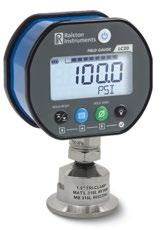
Pressure measuring and monitoring near homogenizers, separators, and heat exchangers requires hygienic instrumentation that can tolerate vibrations, pulsations, wide temperature and humidity changes, and processes that require hot caustic cleaning solutions and acid rinses.
Ralston Instrument’s digital LC20 Diaphragm Pressure Gauge is an ideal solution. With an IP67 rating, an ultra-smooth diaphragm surface, and hygienic triclamp connections that allow the gauge to be steamed or cleaned in place,
46 Oct • Nov • Dec 2022 Cal Lab: The International Journal of Metrology
it
The 4-channel M8199B system provides research engineers the speed, bandwidth, precision and flexibility to meet the challenges of next-generation applications. Credit: Keysight
NEW PRODUCTS AND SERVICES
maintains impressive ±0.1% full scale accuracy in the abusive environments common to the food & beverage, pharmaceutical and biotech industries.
The LC20 Diaphragm Pressure Gauge allows you to perform logging and live viewing of pressure over USB or wireless. Choose from among 15 engineering units or add your own custom units using the included FieldLab software. It’s available in 11 pressure ranges, 5 psi / 35 kPa to 15,000 psi / 100 Mpa, a compound vacuum/pressure gauge from -/+15 psi, and a digital vacuum gauge measuring up to 30 inHg / 760 mbar.
With the LC20 sanitary gauge you’re guaranteed safe, contamination-free pressure measuring and monitoring every time. For more information, visit: https://www. ralstoninst.com/cl-sg
Calculator for Physical Humidity Quantities and Pressure Dew Point
The new Humidity Calculator by E+E Elektronik computes all relevant humidity-related parameters as well as the pressure dew point.
(Engerwitzdorf, 3.8.2022) With the Humidity Calculator by E+E Elektronik, complex humidity calculations can be performed easily and in real-time. This free calculation tool works online in any recent browser and can also be installed as an app on smartphones or a PC. Up to 15 humidity-related parameters can be computed with the practical calculation program. In addition, the E+E Humidity Calculator features a separate calculation mode for determining the pressure dew point.
Humidity calculation including measurement uncertainty
Based on three known physical quantities (pressure, temperature, and a humidity measurand), the E+E Humidity Calculator computes up to 15 humidity-related parameters such as the dew point, frost point, absolute humidity, enthalpy, etc. A significant difference to other humidity calculators is that the E+E Humidity Calculator also takes the measurement uncertainty into account and therefore ensures particularly practical results.
In addition to computing and converting physical humidity quantities, the E+E Humidity Calculator can also be used to simulate the behavior of the humidity values as pressure and temperature conditions change. For realistic calculations, air and 10 other gases (including argon, CO2, helium, and methane) can be selected as the carrier medium.
The formulae for conversion, including computing the uncertainty, are based on the common humidity theories and have been validated by the accredited E+E Elektronik calibration laboratory.

Practical dew point calculator
In addition to calculating the humidity, the E+E Humidity Calculator features a separate calculation mode for computing the dew point in compressed air systems.
This makes it easy to determine the change in dew point temperature in relation to the gas pressure.
User-friendly and functional
The E+E Humidity Calculator is easy and intuitive in use, and it offers a rich set of useful features. For example, the measurement units of the physical quantities can be converted from SI to the US system of units with just one click, or individually defined for each physical quantity. Users can adapt the list of calculated physical quantities to suit their own needs by displaying or hiding individual lines. The computation results can be exported as PDF or Excel files and also sent via e-mail. A click on the Reset button clears all calculations and restores the initial list of measurands.
The E+E Humidity Calculator is accessible on humiditycalculator.epluse.com
MI 6314A Precision Current Divider
November 17, 2022 – Measurements International is pleased to announce the release of a new current divider to replace shunt technology. The 6314A is a 1000:1 Current Divider that works on the world-renowned MI Resistance Bridge and Extenders principal. The 6314A operates at currents up to 3000 A.
Traditional Current Shunts suffer from temperature stability and power coefficient issues that greatly affect the user’s ability to make accurate measurements. The current transformer used in the 6314A has no such issues. The 6314A does not have any uncertainty due to power and temperature and does not require any stabilization time that traditional shunts have.
By eliminating some of the higher uncertainty contributions, measurement experts can now lower uncertainties in highcurrent measurements.
System Features Include
• No stabilization period
• No power coefficient
• No temperature coefficient
• DC and AC operation
• 3000 A Max Current DC
• 1000:1 Range
For more information: https://mintl.com/products/6314aprecision-current-divider/
Cal Lab: The International Journal of Metrology
47 Oct • Nov • Dec 2022
The Hidden Cost of Hardware Upgrades
Michael Schwartz Cal Lab Solutions, Inc.
For years, I have been advocating and teaching the advantages of Object Oriented Programming (OOP) and why we, in the metrology industry, need to move away from scriptbased programming for automation. This often involves explaining to managers and other software developers the costs associated with maintaining multiple procedures for a given Unit Under Test (UUT) and how approaching the development problem from an OOP perspective will save time and money.
The conversation would go something like this: If you write each procedure based on the standards used, you would need six procedures for a given DMM. A typical DMM would have 5700A, 5720A, 5730A, 5500A, 5520A, and 5522A versions – and those are just the Fluke calibrators; there are also the Wavetek, Transmille, and Meatest calibrators. The response I usually get is, “We only have one 5720A and two 5520As.”
The problem most labs don’t understand is the question is not “What do you currently have in your lab?” The real question is, “What are your current and projected software development costs?” Do you understand how costs can increase exponentially?
Now, there are some new calibrators on the market. Last year, Fluke, Transmille, and Meatest introduced new calibrators to the market. And to support them in a scripting language like Fluke MET/CAL ®, a new calibration procedure for each calibrator will need to be created.
Fluke introduced the Fluke 5560A, 5550A, and 5540A; three new procedures for each DMM. Not to
mention oscilloscopes because there is also a scope option available for these new calibrators. Transmille has the 4010A, while Meatest has the 9010, and the 9010+. That is a total of six new calibrators your calibration lab may need to support.
No lab has all the calibrators, but every lab has some subset of the above-mentioned calibrators. Most labs have at least two different calibrators in their labs now. And in the next 5 to 10 years, they will replace one or more of them with one of the above new models introduced this year. Meaning they will have to expand their library of procedures!
There are thousands of procedures that will need to be modified. Then tested, validated, and QA approved, equivalent to hundreds of thousands of man-hours in procedure development and testing for each new calibrator.
Every calibration procedure that uses a multi-function calibrator now needs to be updated. Yes, for many, it will only take a few minutes. But those minutes add up to months of work. Not to mention, new procedures will require a new calibrator version plus one or more legacy calibrator versions, again requiring more man-hours!
So the question is not, “What calibrators do you have in your lab now?” The question is “Does your software support the Hardware of the Future?” Is the software Future Proof?
Having that same conversation with the same managers, now they are understanding the software development cost of adding new hardware. Now they understand the hidden cost of software development
is three times or more than the cost of the hardware.
This is one of the reasons why I created Metrology.NET®. It is truly future-proof. It allows the operator to choose the standard being used at the time of calibration. Simply add a driver for a new calibrator like the Fluke 5560A 9010 or Transmille 4010 and use them in place of a Fluke 55xx calibrator with zero code rewrites.
This is one of the advantages of any well-modeled Object Oriented Programming application. Using the “Prototype” pattern, the programming language allows the developer to create a prototype of a multi-function calibrator that works with any hardware; allowing the operator of the software to choose the specific hardware at the time of calibration, as long as it matches the prototypes’ requirements.
How the prototype pattern works in Metrology.NET ®, is really quite simple. First, a driver is created and tested for the new calibrator. The driver is written to comply with the prototype patterns requirements for a multi-function calibrator. Once the software is tested, the new driver is added to the workstation’s driver directory. It’s really that simple.
There will always be a software cost when adding new hardware to a calibration lab, but that cost doesn’t have to be outrageously expensive. You don’t need to rewrite your entire library, run every procedure, then QA every UUT. The process can be as simple as testing the new driver, double-checking the uncertainties, and adding the driver to the workstation. This can all be done with zero changes to the UUT’s Test Procedure.
48 Oct • Nov • Dec 2022 Cal Lab: The International Journal of Metrology
CORNER
AUTOMATION
10th Symposium on Temperature (ITS10)
10th International Temperature Symposium Disneyland in Anaheim, California USA April 3 - 7, 2023

Thermodynamic Thermometry
Radiation Thermometry
Temperature Scales
Platinum Resistance Thermometry Base-Metal, Nobel Metal Thermocouples W-Re / Refractory Thermocouples
Temperature Fixed Points Humidity and Moisture Metrology Medical and Biological Thermometry Electronic and Noise Thermometry Thermal Imaging (Quantitative)
Program Inquiries:
Dynamic and Transient Thermometry Space and Astrophysics Thermometry Harsh Environment Thermometry Instrumentation and Data Analysis Environmental and Climate Thermometry Temperature Control Calibration Methods and Uncertainties Food Processing Thermometry Photonic / Fluorescence Thermometry Cryogenic Thermometry Semiconductor Process Thermometry
its10@nist.gov

https://its10.msc-conf.com

The International Temperature Symposia have taken place approximately every 10 years since 1919. These Symposia provide opportunities for the presentation and publication of work related to the measurement and control of temperature, with topics ranging from fundamental research on temperature scales to practical measurement solutions in a variety of practical fields.
The 10th International Temperature Symposium will be held at the Disneyland Hotel Conference Center from April 3rd to 7th, 2023, in conjunction with the Measurement Science Conference 2023, along with a combined technology exhibit floor show.
60 Seconds. 10,000 PSI. Fast, Portable, and Reliable. The new Additel 762 features fully automatic pressure calibration like you’ve never seen before. www.additel.com

