
11 minute read
FWPCOA Training Calendar

Continued from page 38 of total trihalomethane (TTHM) contaminants in distribution systems. S Digiano and Zhang (2004) developed a water quality model to simulate bacterial spread and regrowth in water distribution systems. S Islam and Karney (2010) developed a water quality model to simulate release and transport of lead in distribution systems. S Burkhardt et al. (2017) developed a water quality model to simulate fate and transport of arsenic in a real-world water distribution system serving 78,000 customers. S Walski (2019) employed a water quality model to simulate disinfectant residual concentration in distribution systems to comply with water quality regulations.
The American Water Work Association (AWWA) Manual M32, Computer Modeling of Water Distribution Systems, describes the applicability of water quality models to predict contaminant concentrations within distribution systems.
Advertisement
Water Quality Modeling
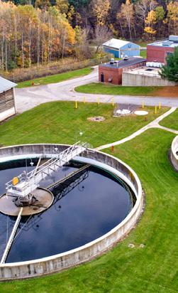
Due to the presence of PFOA within the drinking water sources and the water distribution system serving a community, water quality modeling was performed. The public water system consisted of several groundwater wells, water storage tanks, booster stations, and over 150 mi of water distribution mains. The water distribution system serves over 7,500 water service locations, composed of residential, municipal, commercial, and industrial properties. Water quality modeling was used to estimate the likely historical PFOA concentrations that occurred throughout the water distribution system and determine if PFOA concentrations supplied to residential water system customers, over time, likely met or exceeded threshold values.
This information can be used to help identify residential customers who potentially qualify for medical monitoring. To simulate PFOA concentration within the distribution system, WaterGEMS by Bentley was used. WaterGEMS is one of the commonly used software packages that can provide direct capabilities to assess impacts of contamination events (EPA, 2005).
Water Quality Model Development
The foundation of water quality models is hydraulic models, which simulate the flow quantity, directions, and pressures in water distribution systems. To build a hydraulic model, pipe network properties, topographic information, water use, and operation controls are required. A water quality model determines movement of constituents and travel times through the distribution system. To develop a water quality model, water quality boundary conditions and reaction rates should be defined.
Hydraulic Model
To build the hydraulic model, the WaterGEMS model builder was used to import spatial and attribute information for the pipes, wells with constant speed well pumps, booster pumps, and storage tanks from geographic information system (GIS) shapefiles to the model. In general, attribute information for each pipe included diameter, material, installation date, and active topology status. Inside pipe diameters were estimated based on pipe materials, pipe standards, and nominal diameters. The Hazen-Williams equation was used in the model to calculate frictional energy loss throughout water distribution system piping. The Hazen-Williams coefficient (C) values were determined for various pipe materials and diameters and included consideration of years in service. Model junctions were assigned ground elevation data using the WaterGEMS Terrain Extractor (TREX) tool, which were extracted from a digital elevation model.
System water demands included nonrevenue water (NRW) use and customer water use. The NRW was the difference between water production and total customer water use and it was estimated to be equal to a small percentage of the annual water supply that included leakage and water system flushing, etc. Average customer water use was estimated by analyzing billing records. Customer water use was spatially distributed to the model pipe nodes by geocoding the customer physical addresses and using the nearest pipe method. Demand alternatives were created in the model by globally modifying the overall water usage to equal the actual customer water usage for each year.
To determine well operations during a given day, well run time data were used. To translate this information into the model, a relative speed pattern for each well pump was created for each day. If a well had a production value greater than zero on a given day, the relative speed factor for that well was set to 1 for the duration that the well operated on during that day; for the remainder of the day, the relative speed factor for that well was set to zero. Finally, the well relative speed patterns were adjusted such that the total volume pumped into the system matched with the recorded volume in the well production data. This approach enabled the daily runtimes and daily volumes of water pumped into the water distribution system for each well pump in the model to match the actual or average daily values within specific time periods.
Water Quality Model
To develop the water quality model, the boundary conditions, PFOA decay rate, and water quality mixing were established. The water quality model used the hydraulic model results to route PFOA through each pipe, then mixed at downstream junctions with other inflows into that junction. After mixing, PFOA was conveyed from the junction into its outflowing pipes. This process continued for all pipes and for the duration of the simulation.
Water quality boundary conditions were developed based on the PFOA concentrations in the water in the wells. To establish the well water PFOA concentrations during the simulation, actual PFOA sampling results were used, along with provided groundwater modeling results.
The PFOA reaction rate was set to a negligible value in the water quality model. This is because PFOA is stable in environmental media and doesn’t decay naturally in water (EPA, 2016); additionally, PFOA doesn’t deposit in pipes and the concentration remains constant. The half-life of PFOA in water was estimated to be greater than 92 years (EPA, 2014), which is much longer than the residence time in the water distribution system.
The PFOA diffusion coefficient is very low; consequently, the Peclet number, which is the ratio of advection transport to diffusion transport, is much greater than 1. This indicates that PFOA transport is dominated by advection.
Water quality mixing occurred in the models at junctions and within tanks. A complete mixed solution was used by the model to calculate the concentration in the water entering the downstream pipes at each node. Also, the last in, first out (LIFO) mixing solution was used for the tanks in all model runs based on review of the tank-filling pipe configurations.
Modeling Scenarios
Nineteen extended-period simulation (EPS) modeling scenarios were created to determine the likely PFOA concentrations that occurred in the water distribution system over nearly two decades. For each scenario, the model network alternative was modified to reflect the network that existed in that year (e.g., installing a new water main) based on review of the GIS shapefiles. The properties connected to the system were modified according to the model network alternative modifications for each scenario. This means if a water main was not in service in a given year, the properties connected to that water main, and their demand, would be excluded from the analysis. The water system demand alternative was globally adjusted in the model to equal the actual customer water usage for each year.
A water quality boundary condition alternative was established for each modeling scenario that used actual PFOA sampling and/or groundwater modeling results. To incorporate the daily variations of demand, daily diurnal curves were created for each year using water supply records. Annual average daily demand of the system changed between approximately 2.2 to 2.5 mil gal per day (mgd) over the nearly two-decade time period.
Simulated and Measured Perfluorooctanoic Acid
To determine if the water quality model can reasonably predict PFOA concentrations within the distribution system, simulated PFOA concentrations were compared against historical field-measured concentrations.
Historical PFOA concentrations were available at two locations within the water distribution system (single measurement for each) and at a wholesale customer point of connection (over 150 measurements over a prolonged period of time). A comparison scenario was performed for a one-year period. The overall differences between the simulated and field-measured PFOA concentrations, as well as the similar variations of the simulated and the field-measured PFOA, indicates that the model reasonably represents the operations of the system and transport of PFOA.
Exposure to Perfluorooctanoic Acid Concentrations
Epidemiologic studies indicate that individuals consuming water containing PFOA at concentrations and durations sufficient to increase the blood serum PFOA concentration by a threshold value or more are at increased risk of adverse health effects caused by exposure to PFOA. The expected blood serum PFOA concentration due to water consumption can be calculated using the pharmacokinetic model (Bartell, 2017):
Ct =C(t-1) e-k + W t S (1- e-k)
where C t is an individual’s serum PFOA concentration on day t, k is the daily PFOA excretion rate constant, Wt is the tap water PFOA concentration on day t, and S is the steady-state ratio that shows the average amount of increase in the serum PFOA concentration for each unit increase in the water concentration.
Using the pharmacokinetic model, a table was provided for different exposure characteristics that are expected to increase Continued on page 42
APPLY TODAY
888.621.8156 recruiting@wright-pierce.com wright-pierce.com/careers

JOIN OUR TEAM
Join a firm made up of 300+ employees who are passionate about making a difference in the world.
Own your career with stock ownership, profit sharing plans, and competitive salaries/benefits.
Advance your career with opportunities to work on and lead award-winning treatment, distribution, source, and planning projects. Balance your career working for a familyfriendly firm with flextime, four-hour Fridays, and a hybrid work environment.
Wright-Pierce has opportunities for Project Managers, Lead Project Engineers, and Project Engineers.
Continued from page 41 the serum PFOA concentration by the threshold value. The table indicated the number of days of water consumption needed at each integer water PFOA concentration from 20 to 70 ppt to reach the serum PFOA concentration threshold value. The exposure characteristic table was used in conjunction with water quality modeling results to identify the residential property ownership periods in which occupants would be expected to be at an increased risk of adverse health effects due to consuming drinking water from the water distribution system.
The water quality model was used to estimate the PFOA concentrations within the distribution system over a nearly twodecade period, and the average daily PFOA concentration within each model pipe was determined by averaging the hourly PFOA concentration values for each day. Using GIS, each served residential property was associated with the nearest model pipe, which allowed the average daily PFOA concentrations for all served residential properties to be determined for each day over the nearly two-decade period. Then, the property ownership period information was used to determine the average daily PFOA concentrations for each property ownership period for served residential properties.
The cumulative number of days during which occupants for each served residential property ownership period likely received drinking water were calculated with average daily PFOA concentration of at least 20 ppt through at least 70 ppt in 1-ppt intervals. The cumulative number of days were compared against the exposure characteristics table to identify the served residential property ownership periods during which occupants likely met or exceeded the combination of drinking water PFOA concentrations and cumulative days of consumption expected to increase their serum PFOA concentrations by the threshold value.
Figure 1 shows an example of what the variations of water PFOA concentrations might look like for a served residential property over the nearly two-decade period. For this example, the served residential property is assumed to have four owners during the period of interest. In this example, the analysis would show that during the third ownership period, the occupants were expected to experience serum PFOA concentration greater than, or equal to, the threshold value.
Summary
Water quality modeling was performed to estimate historical PFOA concentrations that occurred within the water distribution system over 20 years. Comparison between the simulated and field-measured PFOA concentrations showed that the model reasonably represents the operations of the system and propagation of PFOA within the distribution system. The water quality modeling results were used to develop a matrix for combination of drinking water PFOA concentrations and cumulative days of consumption for each property ownership period for all served residential properties. An exposure characteristic table was used to identify the served residential property ownership periods when occupants would likely be at increased risk of adverse health effects caused by exposure to PFOA.
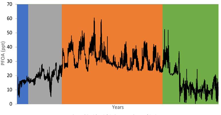

Figure 1. Example of served residential property ownership periods and water perfluorooctanoic acid concentration.
References
• Francis A. DiGiano and Weidong Zhang.
Uncertainty Analysis in a Mechanistic
Model of Bacterial Regrowth in
Distribution Systems. Environ. Sci.
Technol., 38, 5925–5931, 2004. • Md. Monirul Islam and Bryan W. Karney. A
Transient Model for Lead Pipe Corrosion in Water Supply Systems. 2010. • Jonathan B. Burkhardta, Jeff Szaboa, Stephen
Klostermanb, John Halla. Modeling Fate and Transport of Arsenic in a Chlorinated
Distribution System. Environmental
Modeling and Software. Elsevier Science
Ltd, New York, N.Y. 93(1):322-331, 2017. • Robert M. Clark, Brenda K. Boutin.
Controlling Disinfection Byproducts and
Microbial Contaminants in Drinking
Water. EPA. 2001. • Scott M. Bartell. Online Serum PFOA
Calculator for Adults. Environmental
Health Perspectives. 2017. • Tom Walski. Raising the Bar on Disinfectant
Residuals. Bentley Systems Inc. 2019. • USEPA. Technologies and Techniques for
Early Warning Systems to Monitor and
Evaluate Drinking Water Quality: A Stateof-the-Art Review. 2005. • USEPA. Emerging Contaminants:
Perfluorooctane Sulfonate (PFOS) and
Perfluorooctanoic Acid (PFOA). 2014. • USEPA. Drinking Water Health Advisory for Perfluorooctanoic Acid (PFOA). 2016. S
