6.5 The economic factors influencing international trade

The problem for many Australian businesses is that their operations are relatively small with high average costs per unit of output. This is because they often sell their goods and services in a relatively tiny local, state or national market.

However, if local firms succeed in exporting to the world where the potential market size is 7.9 billion people, rather than just sell in the local Australian market with a population of just 26 million, they are able to profitably produce and gain far greater economies of large-scale production. This also means that local businesses can profitably sell their goods and services at a lower, more attractive, and internationally competitive price. Figure 6.7 shows how average unit production costs come down as business sales and production rise. Costs can be spread far more thinly over increased volumes.

FIGURE 6.7 International trade can increase economies of large-scale production for a business by reducing its average costs of production per unit of output through international trade and exports. 3 High per unit cost 2 Low per 1 unit cost 0 1 2 3 4 5 6 Fewer economies of scale Greater economies of when producing just for the scale when producing local market for a global market A firm’s annual level of production/sales (’000)

A BAnnual average cost per unit of output produced ($) Average cost curve FIGURE 6.8 Due to inefficiencies and relatively small volumes, the local car manufacturing industry has closed down as it cannot compete against cheaper imports. 0 UNCORRECTED PAGE PROOFS

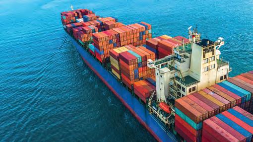
From our earlier studies of the five-sector circular flow model of the economy, we know that the level of aggregate demand or spending on a nation’s goods and services (i.e. AD = C + I + G + X – M), helps to determine the actual level of Australia’s GDP. In fact, foreign spending on our exports of goods and services (i.e. X) amounts to over $480 billion a year. This accounts for between 20–25 per cent of AD and hence also GDP. Without trade, Australia’s economy would be far smaller. In addition, as noted, exports allow local firms to gain greater economies of largescale production where they can profitably sell at lower prices. This makes them more internationally competitive, growing export sales and the overall size of the economy. Exports expand Australia’s employment opportunities and incomes National output and employment levels are directly related. Given the importance of exports as an important determinant of AD and Australia’s GDP, it is not at all surprising that our export sector creates more than 20 per cent of all local jobs. If we can grow exports, this helps to create more employment opportunities, lower the unemployment rate, and reduce the cost for taxpayers and the government of paying welfare benefits. The levels of national output and incomes are also directly related (think of the five-sector circular flow model). By growing Australia’s GDP and hence employment, international trade also enlarges our national income. In turn, this allows us to enjoy higher levels of consumption and better material living standards than otherwise. Increased access to imported resources helps grows Australia’s GDP As we know, the level of national output is ultimately determined by the quantity and quality of natural, labour and capital resources available. While Australia has some types of resources, others are limited or perhaps non-existent. By involvement in international trade, we can export our unwanted surplus resources (e.g. minerals, rural commodities) and use the money gained to pay for imports of things we lack (e.g. raw materials, technology, oil, machinery, appliances) at the lowest possible price. By growing our access to resources, it means that it is possible to expand the economy, lift Australia’s productive capacity, and increase employment and incomes. This is illustrated hypothetically in figure 6.9 using the production possibility diagram. Notice the growth in the size of the production possibility frontier from PPF1 to PPF2. Notice, too, that the combined potential level of output of both goods and services or GDP has risen, following the shift from point A on PPF1 to point B on PPF2. Imports boost our efficiency and keep our inflation rate lower Competition from imports acts as an incentive for local firms to cut their production costs, be more efficient and make their prices more internationally competitive. In turn, consumers benefit from a better range and quality of goods and services that are now sold at lower prices. This increases the purchasing power of incomes and living UNCORRECTED PAGE PROOFS standards. Competition from imports also means that local firms are forced to specialise in producing particular types of goods and services where they have a relative cost advantage. This causes them to use resources more efficiently and gain a bigger output from the same inputs, boosting incomes and living standards.

FIGURE 6.9 The hypothetical effects of international trade on the size of a nation’s production possibility frontier and productive capacity, when it has increased access to imported resources

A nation’s production possibility diagram before and after access to more imported resources

A nation’s original PPF or Production of goods per year (units) Production of services per year 120 180 Point B Point A productive capacity (PPF1), before access to imports of resources- the potential GDP is smaller. A nation’s increased PPF or productive capacity, after access to imports of resources (PPF2)the potential GDP is bigger 6.4.1 The potential benefits for the global economy International trade is beneficial for more nations than only the Commonwealth of Australia. As shown in figure 6.10, it is also beneficial for countries like South Korea, Germany, Canada, South Africa and the European Union, where export trade accounts for over 30 per cent of GDP (and incomes). FIGURE 6.10 Comparing the importance of international trade for selected countries (expressed as a proportion of their GDP) 10 Percentage of GDP Percentage of GDP 0 United States BrazilIndonesiaJapan China (People’s Republic of ) IndiaAustraliaRussiaNew ZealandUnited KingdomFranceTurkeyCanada Italy OECD – AverageSouth Africa KoreaMexicoGermanyEuropean Union 15 20 25 30 35 40 45 50 10 0 15 20 25 30 35 40 45 50 Exports Imports Source: OECD Data, see https://data.oecd.org/trade/trade-in-goods-and-services.htm. 0 UNCORRECTED PAGE PROOFS

By helping to grow the GDP of most countries, international trade brings benefits globally including increased employment opportunities and incomes, lower prices, greater efficiency in the use of limited resources, and better living standards. In some countries like China, it has helped to lift millions out of poverty.

6.4 Activities

Students, these questions are even better in jacPLUS

Receive immediate feedback and access sample responses Access additional questions Track your results and progress

Find all this and MORE in jacPLUS 6.4 Quick quiz 6.4 Exercise

6.4 Exercise 1. Using table 6.3, select any three of the following and explain how international trade can be beneficial. (6 marks) TABLE 6.3 Benefits of international trade

Potential benefits of international trade

2. Explanation of how international trade can be beneficial a. Trade can grow GDP b. Trade can increase economies of largescale production c. Trade can grow access to resources and productive capacity d. Trade can create jobs e. Trade can grow national income f. Trade can boost efficiency As shown in figure 6.9, compared with the European union Australia’s trade as a proportion of GDP is much smaller. Explain how you would expect our lower trade ratio to potentially impact our material living standards. (4 marks) UNCORRECTED PAGE PROOFS

6.5 The economic factors influencing international trade

KEY KNOWLEDGE

• the economic factors influencing international trade Source: VCE Economics Study Design (2023–2027) extracts © VCAA; reproduced by permission. The value of two-way trade (i.e. exports plus imports) reflects the influence of many factors, both domestic and international. In this section, we will investigate just a few of the more important ones. 6.5.1 The exchange rate affects the value of exports and imports The exchange rate at which the currency of one nation (e.g. Australian dollar) is swapped for that of another (e.g. Japanese yen, British pound, European euro, US dollar, Chinese renminbi, South Korean won, Russian ruble, and Singapore dollar). It has a huge effect on the value of a country’s exports and imports. When studying international trade, we need to understand that all transactions involve making payments between countries that mostly have different currencies. So, for instance, Australian exporters of wool want to be paid in Australian dollars, and Japanese exporters of cars want to be paid in Japanese yen. Clearly one currency needs to be swapped for another. This swapping of currencies happens through the foreign exchange market, where buyers and sellers of each currency decide the market price or the exchange rate — the number of units of our currency received when it is swapped for that of another. • When the Japanese need to pay for Australian exports, they have to swap or exchange Japanese yen for Australian dollars. The Japanese sell or supply their yen (increased S) and buy or demand Australian dollars (increased D). Normally, the increased demand for the A$ relative to its supply tends to raise Australia’s exchange rate (a rise in or appreciation of the A$ from ER1 to ER2) while, at the same time, the increased supply of yen relative to its demand drags down the Japanese exchange rate (i.e. causes a fall in or depreciation of the yen). • When Australians need to pay for Japanese imports, we need to sell or supply Australian dollars (increased S) and buy or demand their yen (increased D). The increased supply of our dollars pushes down our exchange rate (i.e. a fall or depreciation of the A$ from ER1 to ER2) while, at the same time, the increased demand for the yen relative to its supply lifts its exchange rate (i.e. causes a rise or appreciation of the yen). Figure 6.11 shows a demand–supply diagram representing the foreign exchange market for the A$. It illustrates that, together, demand and supply determine the exchange rate or price of our currency when it is swapped for other currencies. The four demand–supply diagrams making up figure 6.12 show the effects of changes in the conditions affecting the demand, and changes in the conditions affecting the supply of currencies, on the price or exchange rate for the Australian dollar. • When there are lots of sellers, as shown in graph 1 (i.e. the increase from S1 to S2), and/or few buyers, as shown in graph 4 (the decrease from D1 to D2), the exchange rate falls or depreciates against another currency. • In contrast, having lots of buyers of a currency, as shown in graph 3 (the increase from D1 to D2), and/or fewer sellers, as shown in graph 2 (the decrease from S1 to S2), cause the exchange rate for the A$ to rise or appreciate. UNCORRECTED PAGE PROOFS

FIGURE 6.11 Demand–supply diagram illustrating that demand and supply together determine the exchange rate for our currency

Exchange rate (ER) of price of the A$

Supply > demand for A$

Supply/sales of A$ by sellers

Equilibrium price of A$ or exchange rate (actual ER) Glut of A$ Equilibrium Demand > supply Demand for A$ for A$ by buyers D = S (equilibrium quantity) Quantity of A$ demanded and supplied

A$ depreciates A$ appreciates

Shortage of A$ FIGURE 6.12 Demand–supply diagrams illustrating the effects of changing demand–supply conditions on the value of the A$ Graph 3 — An increase in buying (D1 to D2) strengthens the Australian dollar (A$)

ER2

ER1Price/exchange rate (A$) S1 of the A$ D2 for the A$ D1 for the A$ Q1 Q2 Quantity of A$ Graph 2 — A decrease in selling (S1 to S2) strengthens the Australian dollar (A$) ER2 ER1Price/exchange rate (A$) S2 of the A$ S1 of the A$ D1 for the A$ Q2 Q1 Quantity of A$ Graph 4 — A decrease in buying (D1 to D2) weakens the Australian dollar (A$) ER1 ER2

Graph 1 — An increase in selling (S1 to S2) weakens the Australian dollar (A$) ER1 ER2 Price/exchange rate (A$) S1 of the A$ D1 for the A$ D2 for the A$ Q2 Q1 Quantity of A$

Price/exchange rate (A$) S1 of the A$ S2 of the A$ D1 for the A$ Quantity of A$ Q1 Q2 UNCORRECTED PAGE PROOFS As shown in table 6.4, there are many factors that can alter the conditions of demand (D) and the conditions of supply (S) for the A$ in the foreign exchange market. In turn, they can cause the price of the A$ to either appreciate or depreciate.