18 minute read
4.9 Aggregate demand — its meaning, importance and factors affecting its level and economic activity


KEY KNOWLEDGE
Advertisement
• the relationship between the business cycle and economic indicators
Source: VCE Economics Study Design (2023–2027) extracts © VCAA; reproduced by permission. Mention has already been made that as the economy travels along the business cycle from boom, to slowdown, recession and recovery, the level of economic activity changes. This alters economic conditions and will be reflected in various indicators, some of which are summarised in table 4.5. Starting with some key indicators in column 1, we see how these change over the business cycle during the boom, slowdown, recession, and recovery. Column 1 also describes what the ideal statistic may be for an economy enjoying domestic economic stability. This serves as a benchmark for other conditions.
TABLE 4.5 The relationship between the business cycle and key economic indicators
Common indicator 1 — In a boom Phase of the business cycle 2 — In a slowdown 3 — In a recession 4 — In a recovery
The growth rate in economic activity reflected in AD and
GDP
(The ideal rate of increase in AD and
GDP is an average rise of around 3% rise per year). In response to excessively strong spending/AD and low stocks of unsold goods and services, economic activity/GDP eventually become unsustainably rapid (e.g. perhaps rising by an average of 5% or more per year). In response to gradually weaker spending/AD and reduced orders for goods and services, the growth in economic activity/GDP starts to slow (e.g. perhaps a rise of only 1–2% per year). In response to deficient spending/AD, reduced orders and high stocks of unsold goods and services, output is cut and economic activity/GDP is negative over at least 2 consecutive quarters (e.g. perhaps a fall of -2% per year). In response to stronger spending and new orders, and lower stock levels, firms lift output and the growth in economic activity/GDP starts to accelerate (e.g. perhaps a rise of 1–2% per year).
Unemployment rate
(The ideal rate that is described as full employment — that is, around 4.0–4.5% of the labour force is unemployed). In response to very strong spending/AD and higher production, the unemployment rate falls to very low levels causing labour shortages (e.g. perhaps with only 3% of the labour force unemployed). In response to slower spending/AD and lower production, the unemployment rate starts to rise (e.g. perhaps with 5% of the labour force unemployed). In response to deficient spending/AD and cuts in production, the unemployment rate rises quickly to high levels (e.g. perhaps with 7% or more of the labour force unemployed).
In response to stronger spending/AD and rising output, the unemployment rate gradually starts to fall (e.g. perhaps with 5% of the labour force unemployed). (continued) UNCORRECTED PAGE PROOFS
Common indicator Phase of the business cycle
1 — In a boom 2 — In a slowdown 3 — In a recession 4 — In a recovery
Inflation rate
(The ideal rate that is seen as low inflation is an average rise in consumer prices of between 2–3% per year). In response to excessively strong spending/AD that is beyond the economy’s capacity, there are widespread shortages of goods and services, so consumer prices rise quickly (e.g., perhaps 5% per year or more). In response to slower spending/AD and the gradual disappearance of shortages of goods and services, inflation starts to slow (e.g. perhaps to 3–4% per year). In response to depressed spending/AD, firms are forced to cut or discount their prices to clear rising stocks of unsold goods, causing inflation to slow or become negative (e.g. perhaps a rise of only 1% per year or even -1% per year). In response to gradually strengthening levels of spending/AD and falling stocks of unsold goods, inflation gradually starts to increase (e.g. perhaps rising by around 2–3% per year).
Resourceseses Resources 4.7 Activities
Receive immediate feedback and access sample responses Access additional questions Track your results and progress
Find all this and MORE in jacPLUS 4.7 Quick quiz 4.7 Exercise
4.7 Exercise 1. Examine the hypothetical data for an economy for four separate financial years. (4 marks) TABLE 4.6 Hypothetical data relating to economic conditions in a country
Year 2020–21 2022–23 2024–25 2026–27 Rate of change in economic activity/GDP (%)
-1.9 3.0 7.1 2.0 Unemployment rate (%) 9.4 4.3 2.8 5.1 Inflation rate (%) -0.9 2.8 6.1 1.9 In terms of the business cycle, classify the most likely type of economic situation in each of the following years, explaining your reasons: UNCORRECTED PAGE PROOFS a. 2020–21 b. 2022–23 c. 2024–25 d. 2026–27.
4.8 BACKGROUND KNOWLEDGE: Overview of factors that may affect Australia’s level of economic activity
BACKGROUND KNOWLEDGE
• An overview of aggregate supply and aggregate demand factors that can affect the level of economic activity and domestic macroeconomic conditions There are two main reasons why the level of economic activity may rise or fall. Over the short-term, there are changes in aggregate demand factors, while in the longer-term, there are changes in aggregate supply factors. It is also possible for some factors to have an effect on both aggregate demand and aggregate supply. These ideas are illustrated in figure 4.11.
FIGURE 4.11 Overview of factors affecting Australia’s rate of economic activity Influences on Australia’s level of economic activity Aggregate demand factors:
Aggregate demand factors affect total spending on
Australian-made goods and services (AD = C + I + G +
X – M) over the short-term, determine the actual rate of economic activity and the extent to which the nation’s productive capacity is used.
Aggregate demand factors may involve changes in ... 1. Disposable income 2. Levels of consumer confidence 3. Levels of business confidence 4. Bank interest rates on deposits and loans 5. The exchange rate for the A$ 6. Overseas economic conditions 7. Growth rate in population size 8. Rates of income tax.
Aggregate supply factors: Aggregate supply factors affect Australia’s productive capacity (PPF) or the potential longer-term rate of growth in the level of economic activity. They change the ability and/or willingness of producers to make or supply goods and services. 1. The quantity of resources available and how efficiency these are used 2. Production costs including wages, materials, interest rates on credit, and utility charges 3. Business profitability and whether firms expand or close 4. Climatic events 5. Pandemic lockdowns and disruptions to supply chains 6. Some government economic policies including rates of company tax, education, and infrastructure projects. Aggregate supply factors may involve changes in ... • Aggregate demand factors or conditions influence the total value of spending on a nation’s goods and services. They can be very changeable especially over the short-term and cause AD to rise or fall: • Stronger aggregate demand factors cause the value of total spending to accelerate (shown as flow 3 on the circular flow model), along with the levels of economic activity or GDP (flow 4), employment, incomes, and inflation. • Weaker aggregate demand factors cause total spending to slow (flow 3 on the circular flow model), along with the levels of economic activity or GDP (flow 4), employment, incomes, and inflation. • Aggregate supply factors influence the economy’s long-run productive capacity and potential level of UNCORRECTED PAGE PROOFS
GDP. They can change the conditions that alter the ability and/or willingness of producers to supply goods and services: • More favourable aggregate supply conditions make producers more willing and/or able to expand productive capacity and hence increase the potential rate of economic activity. • Less favourable aggregate supply conditions cause producers to become less willing and/or able to supply, contracting productive capacity and the potential rate of economic activity.
Figure 4.12 (the five-sector circular flow model) shows how these two sets of factors can impact the economy. Aggregate supply factors especially affect the size of flow 1 (i.e., the quantity and quality of resources available that in the long-term affect the potential level of production), while aggregate demand factors change the size of flow 3 (i.e. total value of spending on a nation’s goods and services) and the extent to which productive capacity is used.
FIGURE 4.12 How changing aggregate supply and demand factors can impact economic activity and conditions generally Flow 2 = total incomes paid (demand for resources) Flow 1 = supply of resources to businesses Flow 3 = AD = C + I + G + X – M Private consumption spending (C) LEAKAGES = INJECTIONS = S + T + M I + G + X (act as a brake) (act as an accelerator)
Flow 4 = production (i.e. supply) of goods and services (GDP) BUSINESS SECTOR
Private saving (S) Private investmentFINANCIAL SECTOR spending (I) Government tax GOVERNMENT SECTOR Government (T) spending (G)
Import Export spending (M) OVERSEAS SECTOR spending (X)
Aggregate supply/ Aggregate demand productive capacity is is affected by:affected by: • consumer confidence • quantity and efficiency • business confidenceof all resources • disposable income• profitability • interest rates • production costs • population growth• microeconomic policy • tax rates • wage costs • exchange rate for A$• cost of credit • overseas economic • tax rates on firms activity• seasonal factors • government budget• participation and strike • commodity prices rates • savings levels. • climatic conditions • an ageing population. HOUSEHOLD SECTOR
Resourceseses Resources 4.8 Activities
Receive immediate feedback and access sample responses Access additional questions
Track your results and progress Find all this and MORE in jacPLUSUNCORRECTED PAGE PROOFS
4.8 Exercise
1. Identify and outline the two main determinants of economic activity.
(2 marks)
2. Define the following terms: a. aggregate supply b. aggregate demand.
(1 mark)
(1 mark)
3. Identify and outline the main factors that are affected over the following time spans. a. The short-term rate of economic growth. (2 marks) b. The long-term rate of economic growth. (2 marks) Fully worked solutions and sample responses are available in your digital formats. 4.9 Aggregate demand — its meaning, importance and factors affecting its level and economic activity KEY KNOWLEDGE • the meaning and importance of aggregate demand and its components • the factors that may affect the level of aggregate demand and the level of economic activity Source: VCE Economics Study Design (2023–2027) extracts © VCAA; reproduced by permission. When we see newspaper headlines about the latest recession or boom, we realise that Australia’s rate of economic growth can alter quite suddenly. This is often the result of changes of aggregate demand or the decisions made by households, businesses, and governments about their overall level of spending on Australianmade goods and services. 4.9.1 The meaning and importance of aggregate demand Aggregate demand (abbreviated as AD) represents the total value of all spending by households, businesses, and governments, on finished Australian-made goods and services measured over a period of time. It is made up of various components or types of spending: • Private or household consumption spending (C) on day-to-day purchases PLUS • Private business investment spending (I) on physical capital goods PLUS • Government spending on goods and services for the community PLUS • Foreign spending on our exports of goods and services (X) MINUS our spending on imports We can express this as follows: AD = C + I + G + X – M. Thinking of the five-sector circular flow model, the value of AD can rise or fall due to changes in the total value of leakages (i.e. S + T + M) relative to the total value of injections (i.e. I + G + X). Over the short-term, changes in the value of AD (think of flow 3) determine the level of economic activity (think of the business cycle model and flow 4 on the circular flow model), inflation, unemployment, and incomes. They also dictate the extent to which the economy’s productive capacity or potential output is used (think of the production possibility diagram and the PPF). Clearly, AD is one of the most important variables in the UNCORRECTED PAGE PROOFS economy.
4.9.2 How aggregate demand factors affect the level of AD and economic activity
The level of AD (C + I + G + X – M) and economic activity over the short-term is determined by the strength or weakness of aggregate demand factors or conditions. These might include changes in the following: • the level of household disposable income • the level of consumer confidence or pessimism of households about future employment and income prospects • the level of business confidence about the future sales and profits • the impact of changes in budget taxes and government spending • the level of interest rates paid to banks by those people borrowing credit to finance their spending • the value of the Australian dollar when it is swapped or exchanged for other currencies • general economic conditions overseas (e.g. booms or recessions) in countries to whom we export • the size and growth rate of our population. Let’s take a closer look at how these aggregate demand factors can affect each of the components of spending that make up AD (i.e. AD = C + I + G + X – M). Aggregate demand factors affecting household consumption spending (C): Private consumption spending (C) by Australian households on food, clothes, electrical goods, entertainment, and holidays, for example, is the biggest single component of AD. As a result, it can have a huge effect on total spending. A rise in C for instance would directly stimulate AD (flow 3 on the circular flow model), economic activity, GDP (flow 4), employment of available resources (flow 1) and incomes (flow 2), while reduced spending slows economic activity. As summarised in table 4.7, the value of C can be affected by changes in several aggregate demand factors:
TABLE 4.7 Aggregate demand factors that can affect the level of private consumption spending
Disposable income Household disposable income per head represents money available for spending per person, after the payment of tax and the receipt of any government welfare benefits. A drop in disposable income per head, for example, tends to slow private consumption, while higher disposable income accelerates consumption spending.
Consumer confidence Consumer confidence is the degree of optimism or pessimism about future household incomes and employment prospects. Greater optimism leads to stronger consumption spending and reduced savings, while general pessimism, slows consumption.
Interest rates Interest rates received by households on their bank savings deposits, or those to be paid on credit borrowed from the banks, affect both the level of savings and spending. Higher interest rates encourage savings and discourage borrowing to buy expensive consumer items such as a house or car, while lower interest rates help to lift consumption spending.
Rate of population growth
The rate of population growth (i.e. the excess of births over deaths and immigration levels) influences consumption spending. For instance, a slower Permission clearance pending UNCORRECTED PAGE PROOFS growth in population tends to slow consumption and AD.
Government budgetary policies
Government budgetary policies affect the levels of tax, government spending and other outlays. Cuts in personal income tax rates, for example, can help to increase disposable income and hence consumption spending.
Businesses make spending decisions that affect AD and the level of economic activity. For instance, as an injection on the circular flow model, higher level of private investment spending (I) by businesses on new plant equipment such as computers, factory buildings and trucks, would tend to increase AD, economic activity, GDP, employment and incomes, while reductions have the reverse effect. As shown in table 4.8, the level of I can reflect the influence by changes in various aggregate demand conditions.
TABLE 4.8 Aggregate demand factors that can affect the level of private business investment spending
Business confidence
The level of business confidence or optimism signals expectations about the level of future sales and profits. Business pessimism leads to reduced investment spending on new plant and equipment, while optimism leads to increased investment spending. Interest rates Interest rates charged by banks on loans to firms can alter levels of private investment spending. Higher interest rates tend to discourage investment spending on new equipment because it becomes dearer for firms to borrow and repay credit, while lower rates help to encourage investment spending.
Company tax rates
Company tax rates affect the after-tax profits of businesses. Lower tax rates for businesses help to lift after-tax profits and hence encourage new investment spending designed to expand operations. Rises in tax rates have the opposite effect and slow AD. Here, weaker aggregate demand conditions, perhaps reflecting increased business pessimism, higher interest rates on borrowed credit by firms, rises in company tax rates or rising levels of unsold stocks of goods, would all tend to slow I and reduce AD and the rate of economic growth, leading to a slowdown. In contrast, stronger aggregate demand conditions would tend to increase the level of I and AD, along with economic growth (GDP), employment and incomes. Aggregate demand factors affecting government spending (G) Australian government spending (G) and other outlays on the provision of goods and services community (e.g. health, transport, education, defence and childcare) represents an injection on the circular flow model that can alter the levels of AD. For example, increases in the value of G in the budget tend to boost AD, economic activity, GDP, employment, and incomes, while cuts in G slow AD. Table 4.9 shows that the level of G can be affected by a range of aggregate demand conditions:
TABLE 4.9 Aggregate demand factors that can affect the level of government spending
The level of unemployment The level of G often increases when the unemployment rate rises because, through this approach, the government can help lift AD and reduce the severity of a recession. In reverse, during inflationary booms, the government may slow its spending to stabilise the economy.
The level of inflation The level of G often decreases or slows when inflation is rising because this helps the government restrain AD and reduce shortages of goods and services that cause inflationary pressures.
The speed of population growth
The level of G often rises faster when population growth is more rapid following a rise in the birth rate or an increased level of immigration. This is because more community services are needed. UNCORRECTED PAGE PROOFS
Concern about the level of government debt
If the government spends more than it receives in taxes, it will have to borrow money. This adds to its level of public debt. Concern about high debt levels can act to help slow the level of government spending.
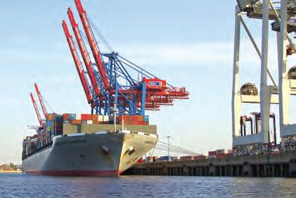
Decisions made by overseas consumers also affect Australia’s AD and level of economic activity. If there is an increase in export spending (X) abroad on Australian made goods and services (e.g. cotton, wool, minerals, manufactured items and travel) as an injection on the circular flow model, this would tend to increase AD, economic activity, GDP, employment and incomes. In reverse, a decrease in the value of our X or injections would have the reverse effects. Table 4.10 shows that changing aggregate demand conditions can influence whether the value of overseas spending on our X rises or falls:
TABLE 4.10 Aggregate demand factors that can affect the level of overseas spending on our exports
The exchange rate or the value of the A$
The exchange rate or the value of the A$ when swapped or converted into other currencies affects the value of our exports. A rising A$ tends to slow our exports because they become dearer to people overseas, while a fall in the A$ makes our exports cheaper, leading to an increase in sales and hence AD.
Overseas economic conditions
Changes in overseas economic conditions, involving booms, recessions, and pandemics can change the value of our exports. For instance, a recession or slowdown abroad among our major trading partners like China, Japan or the US, slows overseas spending on our exports, while a boom overseas tends to raise the value of foreign spending on Australian exports.
Natural disasters Natural disasters and severe weather events in Australia alter our capacity to export. Floods, drought and fires reduce exports of agricultural and mining products. Aggregate demand factors affecting import spending (M) Spending decisions made by local consumers affect AD and the level of economic activity. The level of import spending (M) by Australians (e.g. on oil, computers, business equipment and overseas holidays) represents a leakage on the circular flow. This tends to slow AD, economic activity, GDP, employment and incomes. In contrast, as a leakage, a rise in imports tends to slow spending on Australian goods and services, while a fall in imports lifts AD. The value of import spending can reflect changes in aggregate demand conditions, as seen in table 4.11.
TABLE 4.11 Aggregate demand factors that can affect our level of spending on imports from abroad
The exchange rate or the value of the A$
A fall in the exchange rate for the A$ tends to make imports dearer and less attractive for Australian to purchase, while a rise in the A$ tends to make imports cheaper and more attractive for local consumers. In turn, these changes in leakages affect the level of AD.
Local economic activity If there is stronger consumer and business confidence and high levels of economic activity locally, this often results in more spending on imports where more leakages slow AD. In reverse, weaker conditions and recession here usually mean lower spending on imports.
Consumer and business confidence
Greater household and business optimism locally usually result in more spending on imports, while pessimism tends to lower our spending on imports of goods and services. UNCORRECTED PAGE PROOFS
Our inflation rate relative to that overseas
For instance, higher inflation rates at home make overseas goods and services relatively more attractive, increasing imports and leakages, slowing AD.