equilibrium price and quantity

2.5.1 The law of supply — how changes in price cause a movement along the supply curve

The law of supply simply states that the quantity of a particular good or service that sellers are prepared to supply varies directly (in the same direction) with the change in price, assuming other factors do not change. Hence: • As the price increases, there is an expansion in the quantity supplied, causing a movement upwards along the supply line. • As the price decreases, there is a contraction in the quantity supplied, causing a movement downwards along the supply line. It is hardly surprising that businesses or suppliers behave like this when the quantity supplied contracts or expands along the line following a decrease or an increase in price. This is called a movement along the supply line and occurs because it becomes less profitable for producers to sell their product or service at a lower price, rather than selling it at a higher price. So what would a supply line (representing how sellers respond to price) look like if plotted on a graph where price is located on the vertical axis and quantity on the horizontal axis? Again, imagine there was a competitive market for bananas. Using hypothetical data from the table, figure 2.11 graphically illustrates the relationship that exists between the quantity of bananas supplied and the price, remembering that we have assumed that all non-price factors that might also influence supply are held constant.

FIGURE 2.11 The supply line showing the law of supply for bananas where the quantity supplied varies directly with price Price per The supply line for bananas kg of bananas S1 = Original quantity of bananas supplied each year (’000 kg) $1 1 $2 2 $3 3 $4 $5 5 5 Expansion Price per kg ($) 1 2 3 4 A (from A to B as price increases) Contraction (from B to A as price decreases) 1 2 3 4 5 6 Quantity of bananas supplied each year (’000 kg)

B S1

0 Notice that when we plot the quantity supplied at each possible price on a graph (see figure 2.11), the resulting supply line slopes up and to the right. Here it is again worth remembering that, for simplicity, this basic supply line has been drawn straight rather than curved in shape, as might appear in reality. Either way, the line has a positive slope and visually illustrates the law of supply. • A move upward along the supply line (or curve) from point A to point B is called an expansion in supply and is only caused by a rise in price. In our example, the quantity supplied expands from 2000 kg per year at the price of $2 per kg (point A) to 4000 kg at the higher price of $4 per kg (point B). • In reverse, a move downwards along the supply line (or curve) from point B to point A is called a contraction in supply and is only caused by a fall in price. In our example, supply contracts from 4000 kg per year at a price of $4 per kg (point B) to only 2000 kg per year at the low price of $2 per kg (point A).

4 UNCORRECTED PAGE PROOFS

Again, it is really important to understand that these movements along the supply line (called an expansion or contraction in the quantity supplied) are caused solely by a change in price. And again, we have assumed that all non-price factors that might influence supply have been held constant. We will look at these non-price factors shortly. For simplicity, the supply line for bananas (see figure 2.11) has been drawn as a straight line, even though in the real world it would usually be a concave curve (called a supply curve).

While our example here has been the supply of bananas, the same sort of seller behaviour could be expected for any other good (such as grapes, hot dogs, soft drinks, suncream or deodorant) or service (such as financial, health, educational, gardening or entertainment) in a fairly competitive market.

Resourceseses

Resources Video eLesson Movement along vs. a shift in the supply curve (eles-3505) Interactivity Movement along vs. a shift in the supply curve (int-7880) 2.5 Activities

Students, these questions are even better in jacPLUS

Receive immediate feedback and access sample responses Access additional questions Track your results and progress

Find all this and MORE in jacPLUS 2.5 Exercise 2.5 Quick quiz

2.5 Exercise 1. Describe what demand–supply diagrams show. (2 marks) 2. Describe what is meant by supply. (1 mark) 3. Explain the law of supply. (1 mark) 4. Explain why sellers behave like this. (1 mark) 5. Refer again to the background information on Australia’s electricity market in the applied economic exercises in subtopic 2.4 to answer these questions. The supply of electricity Examine table 2.3 containing hypothetical data showing the original supply of electricity in the market at various prices. TABLE 2.3 The original quantity of electricity supplied at various prices in the market

Possible price per kWh ($)

Original quantity of electricity supplied per day (millions of kWh) at a given price (S1) $0.10 $0.15 10 $0.20 15 $0.25 20 $0.30 25 $0.35 30 5 UNCORRECTED PAGE PROOFS $0.40 35

a. Define what is meant by the supply of electricity. (1 mark) b. Using table 2.3, accurately construct a graph showing the supply line or curve for electricity. (3 marks)

c. Explain the law of supply for electricity, illustrating your response with data drawn from the table. (2 marks) d. Distinguish an expansion in the supply of electricity from a contraction in supply. (2 marks) e. If the price falls from $0.40 to $0.30 cents per kWh, describe what happens to the quantity of electricity supplied using figures to illustrate your answer. Remember to use the correct word reserved for describing this shift along the supply curve. (2 marks) f. If the price falls from $0.30 to $0.10 cents per kWh, describe what happens to the quantity of electricity supplied using figures to illustrate your answer. Remember to use the correct word reserved for describing this shift along the supply curve. (2 marks) g. Other things remaining equal, explain why the supply of electricity expands as the price rises, causing a movement along the supply curve or line. (2 marks)

Fully worked solutions and sample responses are available in your digital formats.

2.6 Determining the market equilibrium price and equilibrium quantity

KEY KNOWLEDGE • the effects of changes in demand and supply on equilibrium prices and quantities

Source: VCE Economics Study Design (2023–2027) extracts © VCAA; reproduced by permission. As we have seen, buyers prefer to purchase at a relatively low price, while suppliers prefer to sell at a relatively high price. This apparent conflict of interest or disagreement is resolved by negotiation and haggling — offer and counteroffer — and the operation of a competitive market. Indeed, there is only one price on which both buyers and sellers agree and are reasonably satisfied. This is called the equilibrium market price. At equilibrium, the quantity demanded exactly equals the quantity supplied, and there is no force for further change. The market is currently stable. As seen in the demand–supply (D–S) graph in figure 2.12, apart from the equilibrium price of $3 per kg of bananas, there is no alternate market price where this compromise can occur. Only at this price are both the quantity demanded and the quantity supplied exactly equal — both demand and supply are equal to 3000 kg per year. At equilibrium, both buyers and sellers are happy with the deal and the market is cleared so there is neither a shortage nor a surplus.

FIGURE 2.12 A demand–supply (D–S) graph showing how the free operation of market forces determines the equilibrium price of bananas Price per kg of bananas D1 = Original quantity of bananas demanded each year (’000 kg) S1 = Original quantity of bananas supplied each year (’000 kg) $1 5 $2 4 $3 3 $4 2 $5 1 1 2 3 4 5

How demand and supply create equilibrium in the market for bananas 1Price per kg ($) 3 4 5 S1 D1 At prices above Pe, there is a glut (i.e. S > D) Pe At prices below Pe there is a shortage (i.e. D > S) E (equilibrium) 2 UNCORRECTED PAGE PROOFS 0 1 2 3 4 5 6 Qe, D = S Quantity of bananas demanded and supplied each year (’000 kg)

The process of actually reaching market equilibrium in a free and competitive market is a simple one: • Prices below the equilibrium. At a very low price for bananas of, say, $2 per kg, equilibrium cannot occur simply because 4000 kg per year are demanded yet only 2000 kg are supplied. An exceedingly low price like this creates a market shortage of 2000 kg, making buyers very unhappy when they go away empty handed. In order for this shortage to be solved, the price of bananas needs to rise. As the price moves upwards, there is a contraction along the demand line for bananas, as well as an expansion along the supply line (the laws of demand and supply apply here) until this market shortage disappears and the market reaches the equilibrium point where the quantity demanded and supplied are exactly equal. • Prices above the equilibrium. Equilibrium is also not possible at an exceedingly high price of, say, $4 per kg of bananas. The problem here is a market surplus or glut of 2000 kg. This arises due to a demand of only 2000 kg, compared with the supply of 4000 kg at that price. Sellers would be most unhappy because they have unsold stock that would perish. In a free and competitive market, this problem would soon disappear as the market price falls. A falling price would cause an expansion along the demand line for bananas while at the same time there would be a contraction along the supply line causing the market surplus to gradually disappear. Market equilibrium would be restored so that the quantities demanded and supplied were again exactly equal. In our analysis so far, we have seen that market forces involving demand and supply determine the actual equilibrium price for bananas. However, the same sort of explanation would also apply to the equilibrium price paid for any type of good or service in a competitive market. All competitive markets basically operate in the same way.

Resourceseses Resources Video eLesson Supply and demand equilibrium (eles-3500) 2.6 Activities

Students, these questions are even better in jacPLUS

Receive immediate feedback and access sample responses Access additional questions

Track your results and progress Find all this and MORE in jacPLUS 2.6 Exercise 2.6 Quick quiz 2.6 Exercise 1. Define the term equilibrium. (1 mark) 2. Outline the circumstances when a market shortage occurs. (1 mark) 3. Outline the circumstances when a market surplus occurs. (1 mark) 4. Refer again to the background information on Australia’s electricity market in the applied economic exercises in subtopic 2.4 to answer these questions. Equilibrium price and quantity in the electricity market Examine table 2.4 containing hypothetical data showing both the original demand for and the original supply of electricity at various prices in the market. UNCORRECTED PAGE PROOFS

TABLE 2.4 The original quantities of electricity demanded and supplied at various prices in the market

Possible price per kWh ($) Original quantity of electricity demanded per day (millions of kWh) at a given price (D1)

Original quantity of electricity supplied per day (millions of kWh) at a given price (S1)

$0.10 35 5

$0.15 30 10 $0.20 25 15 $0.25 20 20 $0.30 15 25 $0.35 10 30 $0.40 35 a. Using table 2.4, accurately construct and fully label a combined D–S graph showing the original demand (D1) and the original supply (S1) curves or lines for the electricity market, along with the original market equilibrium (E1). Your labelling must include an appropriate scale and units for each of the two axes (with both scales rising by regular intervals from zero), along with D1, S1, E1, P1 and Q1. (4 marks) b. In this example, explain what is meant by equilibrium (E1) in the electricity market. (1 mark) c. Looking at the data and diagram, estimate the equilibrium price (P1) for electricity in this market. (1 mark) d. Looking at the data and diagram, estimate the equilibrium quantity (Q1) for electricity in this market. (1 mark) e. Explain why the price of $0.10 per kWh is not the actual equilibrium market price for electricity. Quote figures from the table to illustrate your response. (2 marks) f. Explain why the price of $0.40 per kWh is also not the actual equilibrium market price for electricity. Quote figures from the table to illustrate your response. (2 marks) g. At equilibrium, explain why the price be steady where it neither wants to rise or fall (assuming all other things remain equal or constant). (3 marks) Fully worked solutions and sample responses are available in your digital formats. 2.7 The effects of non-price factors on demand and supply — shifting the D–S curves and changing the equilibrium price and quantity KEY KNOWLEDGE • the effect on demand and the position of the demand curve by non-price factors, including changes in disposable income, the prices of substitutes and complements, tastes and preferences, interest rates, population and demographics, and consumer confidence • the distinction between a movement along the demand curve and a shift of the demand curve • the effect on supply and the position of the supply curve by non-price factors, including changes in the costs of production, technology, productivity, and climatic conditions and other disruptions • the distinction between a movement along the supply curve and a shift of the supply curve Source: VCE Economics Study Design (2023–2027) extracts © VCAA; reproduced by permission. 5 UNCORRECTED PAGE PROOFS Looking around us, we notice that the prices of most goods and services, including bananas, are always changing up and down from week to week and day to day. This is the result of changes in the level of demand relative to the level of supply for each good or service, as buyers and/or sellers react to new non-price microeconomic factors or conditions that affect their economic decisions and the quantity they are prepared to buy or sell at any given price.

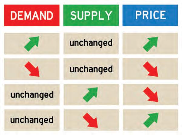
• New non-price demand-side factors or conditions can cause buyers to purchase a greater or smaller quantity of a particular good or service at all possible prices. This will either shift the position of the whole demand line on a diagram horizontally to the right of the original line (showing an increase in the quantity demanded at all possible prices), or to the left (showing a decrease in the quantity demanded at all possible prices). • New non-price supply-side factors or conditions can cause sellers to produce a greater or smaller quantity of a particular good or service at all possible prices. This will either shift the position of the whole supply line on a diagram horizontally to the right of the original line (showing an increase in the quantity supplied at all possible prices), or to the left (showing a decrease in the quantity supplied at all possible prices). By altering the position of the demand line and/or the position of the supply line, changes in non-price microeconomic factors or conditions of demand or supply will bring about a change in relative prices (i.e. the price level of one particular good or service relative to that of another). This change in relative price also has a knock-on effect and alters the relative profits of producing a particular good or service. A higher equilibrium price that makes it relatively more profitable (a positive incentive) will normally attract more resources to be allocated to the production of this product, while a fall in the equilibrium price will usually cause fewer resources to be allocated to the production of this item due to relatively lower profits (a negative incentive). In so doing, it causes scarce resources to be reallocated among competing uses by their profit-seeking owners. 2.7.1 How non-price factors can shift the position of the whole demand curve changing the equilibrium price and quantity Changes in non-price factors can shift the position of the whole demand curve, affecting both the equilibrium price and quantity traded. Figure 2.13 reveals that there are a number of common non-price microeconomic factors or conditions of demand that might either increase or decrease the quantity of a particular good or service that buyers are prepared to demand at a given price. On a demand–supply diagram, these factors or conditions shift the position of the demand line for a good or service horizontally to the right or to the left of the original line.

FIGURE 2.13 Non-price microeconomic factors or conditions that cause the quantity of a good or service demanded at a given price to increase or decrease, shifting the position of the whole demand line Non-price conditions can increase the quantity demanded at a given price (shifting the whole line from D1 to D2 ). Price/unit 20 D1 D2 5 10 15 Quantity This diagram shows an increase in the quantity demanded (D1 to D2) at a price of $20, from 10 units to 15 units.

Non-price conditions can decrease the quantity demanded at a given price (shifting the whole line from D1 to D0 ). 0 20 5 10 15 D0 D1 Price/unit This diagram shows a decrease in the Quantity 0 UNCORRECTED PAGE PROOFS quantity demanded (D1 to D0) at a price of $20, from 10 units to 5 units.

A rise in disposable income (income available for spending after receiving welfare and paying income tax) usually increases the quantity of a good or service demanded at a given price. A fall in disposable income. A fall in disposable income usually decreases the quantity of a good or service demanded at a given price.

An increase in population size. Generally, a rise in population, perhaps due to immigration or higher birth rates, will increase the quantity of most goods or services demanded at a given price. A decrease in population size. Generally, a decline in population, perhaps due to the ageing of the population, might decrease the quantity of some goods or services demanded at a given price (e.g. pop music).

More fashionable and trendy. Over time, some goods and services become more fashionable, perhaps as a result of new technology and slick advertising (e.g. the latest iPhone). This increases the quantity of most goods or services demanded at a given price. Less fashionable. Over time, some goods and services become less fashionable. The quantity demanded by consumers at a given price declines (e.g. DVD players).

A drop in interest rates paid on borrowed credit.

Some people and businesses need to borrow credit from banks and pay interest rates, in order to purchase expensive goods or services. When interest rates are lower and borrowing is cheaper, the quantity of most goods or services demanded at a given price increases (e.g. a house, car or electrical appliances, and holidays).

Higher interest rates paid on borrowed credit.

Generally, higher interest rates will lower the quantity of most goods or services demanded at a given price.

A substitute becomes dearer. Substitutes are a particular good or service that can be easily replaced by another (e.g. margarine is a substitute for butter and cotton for wool) so the price of one affects the demand for the other. For instance, when the price of margarine becomes dearer, the demand for butter is likely to increase. A substitute becomes cheaper. When the price of a substitute product like cotton becomes cheaper, the demand at any given price for the other product like wool decreases, as people switch between products.

A complementary good or service becomes cheaper.

Complementary goods and services are those used or bought at the same time as another item (e.g. cars and fuel). Hence, when the price of one complement falls, the demand for the other complementary good is likely to rise (e.g. a fall in petrol prices leads to a rise in the demand for larger 4WD vehicles).

A complementary good or service becomes dearer.

When the price of one complementary good or service rises, there is usually a decrease in the demand for the other complementary product (e.g. the price of coffee rises and the demand for sugar decreases) at a given price.

Higher levels of consumer or business confidence.

Confidence levels relate to how households and businesses feel about their future economic situations. For instance, when households are feeling more confident or optimistic, they often purchase a greater quantity of some types of goods and services at a given price (e.g. luxury cars and holidays).

Lower levels of consumer or business confidence.

Consumer or business pessimism about the future is often reflected in a decrease in the demand for some types of goods (e.g. appliances and beauty products) or services (e.g. entertainment and restaurants) at any given price.

The onset of summer or winter. In summer, the demand for some products at a given price increases (e.g. ice-cream, surfboards and air conditioners). Furthermore, the onset of winter might see a rise in the demand for other types of goods or services at a given price (e.g. snow skis, cough medicine, doctors, electric blankets, footballs and woollen jumpers).

The onset of summer or winter. The onset of winter might see a decrease in the demand for some goods or services at a given price (e.g. air conditioners). Additionally in summer, the demand for other goods and services at a given price might decrease (e.g. beach towels and insect repellent). UNCORRECTED PAGE PROOFS

New government policies. Sometimes, new government policies can lead to a rise in the demand for particular goods or services. For instance, a rise in government transport spending might bring about an increase in the demand for building and road making materials. Sometimes, too, the government uses cash subsidies or payments as an incentive to encourage households to increase their demand for socially beneficial items (e.g. solar panels and rainwater tanks).

New government policies. Sometimes, new government policies can lead to a decrease in the demand for a socially harmful good or service at a given price (e.g. laws making it illegal for young people to purchase alcohol, or the addition of a tax as a disincentive to purchase a product). New non-price factors can increase the quantity demanded (D1 to D2) at a given price: • When non-price conditions of demand strengthen, increasing the quantity of a particular good or service that buyers are willing to purchase at any given price (e.g. called an increase in demand at $3 per kg for bananas), the whole demand line for the market will shift outwards horizontally and to the right of the original line (a shift from D1 to D2). • Let us return to the example of the banana market as shown in figure 2.13. When the demand for bananas at a given price increases because of new stronger conditions (perhaps due to more consumers wanting a healthy snack; an increase in disposable income; population growth; or successful advertising by banana growers), this shifts the position of the whole demand line horizontally to the right of the original line, from D1 to D2. As a result, there is a rise in the equilibrium price of bananas from $3 (at P1) to $3.50 a kg (at P2). This rise in the equilibrium price is necessary to clear the market shortage (see the triangular area shaded red, where the quantity demanded exceeds the quantity supplied) that would otherwise exist if the price had remained at $3. As the price rises towards $3.50, demand contracts while supply expands (the normal operation of the laws of demand and supply) until the new higher equilibrium price (P2) is reached where demand again equals supply. Notice also that there is a rise in the equilibrium quantity from 3000 (at Q1) to 3500 kg a year (at Q2). These new equilibria will prevail in the market unless non-price conditions of demand again change. New non-price factors can also decrease the quantity demanded (D1 to D0) at a given price: • When non-price conditions of demand weaken, decreasing the quantity of a particular good or service that buyers are willing to purchase at any given price (e.g. a decrease in demand at $3 per kg for bananas), the whole demand line for the market will shift inwards horizontally and to the left of the original line (a shift from D1 to D0). • Returning to the banana market and figure 2.13, when the demand decreases because of new weaker conditions (perhaps due to the onset of winter; advertising by pineapple growers; a drop in income; or poorer quality fruit), this shifts the position of the whole demand line left, from D1 to D0. As a result, there is a fall in the equilibrium price of bananas from $3 (at P1) to just $2.50 a kg (at P0). This fall in the equilibrium price is necessary to clear the market glut or surplus (see the triangular area shaded green, where the quantity supplied exceeds the quantity demanded) that would otherwise exist if the price had remained at $3. As the price drops towards $2.50, demand expands while supply contracts (the normal operation of the laws of demand and supply) until the new lower equilibrium price (P0) is reached where the quantity demanded again equals the quantity supplied. Notice also that there is a fall in the equilibrium quantity from 3000 (at Q1) to 2500 kg a year (at Q0). These new equilibria will prevail in the market unless non-price conditions of demand again change. 2.7.2 How non-price factors can shift the position of the whole supply curve changing the equilibrium price and quantity UNCORRECTED PAGE PROOFS In the same way as buyers react to changing circumstances, sellers also respond to variations in non-price microeconomic factors or conditions of supply. These might either increase or decrease the quantity of a particular good or service that sellers are prepared to supply at a given price. On a demand–supply diagram, these new non-price conditions cause a shift in the position of the supply line horizontally to the right or to the left of the original line. Figure 2.15 shows that there are a number of common non-price supply-side conditions.

FIGURE 2.14 How changes in microeconomic non-price conditions of demand can increase or decrease the quantity demanded at any given price, shifting the whole demand line horizontally and causing the equilibrium market price to either rise or fall

5 4 Price per kg ($) 2 3 1 2 Q0 3 Q2

E0 D0

E1 E2 S1 D1

Price per kg How changes in non-price conditions of demand can cause the equilibrium market price to rise or fall

P2 P1 P0 D2 0 Q1 4 5 6 Quantity of bananas demanded and supplied each year (’000 kg)

D1 = Original quantity of bananas demanded each year (’000 kg) D2 = New increased S1 = Original quantity quantity of bananas of bananas supplied demanded each year each year (’000 kg) (’000 kg)

D0 = New decreased quantity of bananas demanded each year (’000 kg) $0 $1 $2 $3 $4 $5

5 4 3 2 1 4 3 2 1

1 2 3 4 5 6 5 4 3 2 New non-price factors can increase the quantity supplied (S1 to S2) at a given price: • When non-price conditions of supply strengthen or become more favourable, there is an increase in supply or the quantity of a particular good or service that sellers are willing to produce at a given price (e.g. an increase in supply at $3 per kg for bananas). The whole supply line for the market will shift outwards horizontally and to the right of the original line (a shift from S1 to S2). • Let us return again to the example of the banana market as shown in figure 2.16. When the supply of bananas increases due to new, more favourable conditions (perhaps reflecting the effects of ideal growing conditions for farmers, or lower costs and better profits), this shifts the position of the whole supply line outwards horizontally and to the right, from S1 to S2. As a result, there is a fall in the equilibrium price of bananas from $3 (at P1) to just $2.50 a kg (at P2). This fall in the equilibrium price is necessary to clear the market glut or surplus (see the triangular area shaded green, where the quantity supplied exceeds the quantity demanded) that would otherwise exist if the price had remained at $3. As the price falls towards $2.50, supply contracts and demand expands (the normal operation of the laws of demand and supply) until the market comes to rest at the lower equilibrium price (P2). In addition, the equilibrium quantity rises from 3000 kg (at Q1) to 3500 kg a year (at Q2). These new equilibria will continue to exist unless non-price conditions of supply again change. New non-price factors can also decrease the quantity supplied (S1 to S0) at a given price: 1 UNCORRECTED PAGE PROOFS • When non-price conditions of supply weaken or become less favourable, this decreases the quantity of a particular good or service that sellers are willing to produce at a given price (e.g. a decrease in supply at the price of $3 per kg for bananas). This causes the whole supply line for the market to shift inwards horizontally and to the left of the original line (a shift from S1 to S0).

• Let us return yet again to the example of the banana market shown in figure 2.16. When the supply of bananas decreases at a given price due to new, less favourable conditions (perhaps reflecting the effects of severe drought; the effect of a cyclone; or higher production costs for farmers), this shifts the position of the whole supply line horizontally to the left, from S1 to S0. As a result, there is a rise in the equilibrium price of bananas from $3 (at P1) to $3.50 a kg (at P0). This rise in price is necessary to clear the market shortage (see the triangular area shaded red, where the quantity demanded exceeds the quantity supplied) that would otherwise exist if the price had remained at $3. As the price rises towards $3.50, supply expands and demand contracts (the normal operation of the laws of demand and supply) until the market comes to rest at the higher equilibrium price (P0). In addition, the equilibrium quantity falls from 3000 kg (at Q1) to 2500 kg a year (at Q0). These new equilibria will continue to exist unless non-price conditions of supply again change. FIGURE 2.15 Non-price microeconomic factors or conditions that cause the quantity of a good or service supplied at a given price to increase or decrease, shifting the position of the whole supply line 20 5 10 15 Quantity This diagram shows an increase in the quantity supplied (S1 to S2) at a price of $20, from 10 units to 15 units.

Price/unit S1 S2

Non-price conditions can increase the quantity supplied at a given price (shifting the whole line from S1 to S2). Price/unit 20 S0 S1 0 5 10 15 Quantity This diagram shows a decrease in the quantity supplied (S1 to S0) at a price of $20, from 10 units to 5 units.

Non-price conditions can decrease the quantity supplied at a given price (shifting the whole line from S1 to S0).

Resources used by businesses become cheaper.

Businesses need to purchase natural, labour and capital resources in order to make goods and services. These represent production costs. When costs are cheaper, this makes production more favourable and profitable for businesses. It often causes firms to increase their quantity of a good or service supplied at any given price.

Resources used by businesses become dearer. When production costs become dearer for businesses, this is less favourable and profitable for firms, causing them to decrease their quantity supplied at any given price. Disruptions to supply chains due to pandemics, lockdowns or war, can also increase production costs and cut the quantity supplied at a given price. Increased productivity or efficiency. The use of improved technology like automated warehouses, robotics on an assembly line and online trading in an industry, often lifts efficiency, cutting unit production costs. This usually makes firms more willing and able to increase their supply at any given price.

Decreased productivity or efficiency. A drop in the efficiency of workers in an industry, or in the productivity of other resources used, will often lead to higher business costs. This is likely to decrease the supply of a particular good or service at any given price. More favourable climatic conditions. Climatic conditions affect farmers supplying crops. Favourable weather conditions means that more output per hectare can be produced, at lower unit costs. This increases the quantity of some rural commodities supplied (e.g. wheat, beef, barley, fruit and vegetables) at any given price.

Unfavourable climatic conditions. Severe weather events, such as cyclones, floods and drought, tend to 0 UNCORRECTED PAGE PROOFS reduce efficiency and the supply of some fruit, vegetables and other crops. Floods can also hamper mining extraction operations and destroy infrastructure needed to transport minerals to terminals. This can decrease the quantity supplied at a given price.

FIGURE 2.16 How changes in microeconomic non-price conditions of supply can increase or decrease the quantity supplied at any given price, shifting the whole supply line and causing the equilibrium market price to either rise or fall

5 4.5 4 Price per kg ($) 1.5 2 2.5 3.5 1 0.5 1

How changes in non-price conditions of supply can cause the equilibrium market price to rise or fall

S0

S1 S2

Q1 2 4 Quantity of bananas demanded and supplied each year (’000 kg)

Price per kg E0P0 E1P1 E2

P2 D1

Q0 Q2 0

3 5 6

S1 = Original quantity of bananas supplied each year (’000 kg) S2 = New increased quantity of bananas supplied each year (’000 kg) S0 = New decreased quantity of bananas supplied each year (’000 kg) $0 $1 $2 $3 $4 $5

1 2 3 4 5 2 3 4 4 0 1 2 3 4

D1 = Original quantity of bananas demanded each year (’000 kg) 5 4 3 2 16 Resources 3 UNCORRECTED PAGE PROOFS

Resourceseses

Video eLesson Using supply and demand curves to predict price changes (eles-3503)

Students, these questions are even better in jacPLUS

Receive immediate feedback and access sample responses Access additional questions Track your results and progress

Find all this and MORE in jacPLUS

2.7 Exercise 2.7 Quick quiz

2.7 Exercise 1. Giving examples, describe what non-price microeconomic conditions of demand involve. (2 marks) 2. Giving examples, describe what non-price microeconomic conditions of supply involve. (2 marks) 3. Explain how changes in non-price microeconomic conditions affect demand and supply, and the equilibrium market price and quantity traded. 4. Distinguish between a movement along a demand or supply line, and a shift of the whole demand or supply line. (2 marks) 5. Refer again to the background information on Australia’s electricity market in the applied economic exercises in subtopic 2.4 to answer these questions.

Changes in non-price conditions of demand and/or supply in the electricity market

Market theory suggests that the sharp rise in electricity prices, especially over the period from 2008 to 2019, reflects the effects of new non-price microeconomic conditions that have increased the quantity demanded relative to the quantity supplied or available.

Examine table 2.5 containing hypothetical data showing both the original demand (D1) for and the original supply (S1) of electricity at various prices in the market. The table also includes another set of data showing an increase in the quantity of electricity demanded at various prices, reflecting new stronger non-price microeconomic conditions of demand (called D2). These will shift the position of the original demand curve or line (from D1 to D2).

TABLE 2.5 The original quantities of electricity demanded and supplied, plus the new increased quantity demanded, at various prices in the market

Possible price per kWh Original quantity of electricity demanded per day (millions of kWh) at a given price (D1) Original quantity of electricity supplied per day (millions of kWh) at a given price (S1)

New increased quantity of electricity demanded per day (millions of kWh) at a given price (D2) $0.10 35 40 $0.15 30 10 35 $0.20 25 15 30 $0.25 20 20 25 $0.30 15 25 20 $0.35 10 30 15 $0.40 5 35 10 a. Using table 2.5, accurately construct and fully label a combined D–S graph showing the original demand (D1) and the original supply (S1) curves or lines for the electricity market, along with the original market equilibrium (E1). Your labelling must include an appropriate scale and units for each of the two axes (with 5 UNCORRECTED PAGE PROOFS both scales rising by regular intervals from zero), along with D1, S1, E1, P1 and Q1.

On the same graph, plot and label a second demand curve or line (called D2), the new equilibrium price (called P2) and the new equilibrium quantity (called Q2). Notice how the new non-price demand conditions